An Introduction to pytidycensus
pytidycensus is a Python package designed to facilitate the process of acquiring and working with US Census Bureau population data in Python.
This is a port of Kyle Walker’s excelent intro to tidycensus in R - he deserves the credit for this tutorial! I just converted it to Python.
The package has two primary goals: first, to make Census data available to Python users in a pandas-friendly format, helping kickstart the process of generating insights from US Census data. Second, the package streamlines the data wrangling process for spatial Census data analysts. With pytidycensus, Python users can request geometry along with attributes for their Census data, helping facilitate mapping and spatial analysis.
The US Census Bureau makes a wide range of datasets available through their APIs and other data download resources. pytidycensus focuses on a select number of datasets implemented in a series of core functions. These core functions include:
get_decennial(), which requests data from the US Decennial Census APIs for 2000, 2010, and 2020.get_acs(), which requests data from the 1-year and 5-year American Community Survey samples. Data are available from the 1-year ACS back to 2005 and the 5-year ACS back to 2005-2009.get_estimates(), an interface to the Population Estimates APIs. These datasets include yearly estimates of population characteristics by state, county, and metropolitan area, along with components of change demographic estimates like births, deaths, and migration rates.
Getting started with pytidycensus
To get started with pytidycensus, users should install the package and load it in their Python environment. They’ll also need to set their Census API key. API keys can be obtained at https://api.census.gov/data/key_signup.html. After you’ve signed up for an API key, be sure to activate the key from the email you receive from the Census Bureau so it works correctly.
import pytidycensus as tc

tc.set_census_api_key("YOUR_API_KEY")
Decennial Census
Once an API key is set, users can obtain decennial Census or ACS data with a single function call. Let’s start with get_decennial(), which is used to access decennial Census data from the 2000, 2010, and 2020 decennial US Censuses.
To get data from the decennial US Census, users must specify a string representing the requested geography; a vector of Census variable IDs, represented by variables; or optionally a Census table ID, passed to table. The code below gets data on total population by state from the 2010 decennial Census.
import pytidycensus as tc

total_population_10 = tc.get_decennial(
    geography="state",
    variables="P001001",
    year=2010
)

print(total_population_10.head())
Getting data from the 2010 decennial Census
Using Census Summary File 1
  GEOID   P001001 state        NAME
0    01   4779736    01     Alabama
1    02    710231    02      Alaska
2    04   6392017    04     Arizona
3    05   2915918    05    Arkansas
4    06  37253956    06  California
The function returns a pandas DataFrame with information on total population by state, and assigns it to the object total_population_10. Data for 2000 or 2020 can also be obtained by supplying the appropriate year to the year parameter.
Summary files in the decennial Census
By default, get_decennial() uses the argument sumfile = "sf1", which fetches data from the decennial Census Summary File 1. This summary file exists for the 2000 and 2010 decennial US Censuses, and includes core demographic characteristics for Census geographies.
2020 Decennial Census data are available from the PL 94-171 Redistricting summary file, which is specified with sumfile = "pl" and is also available for 2010. The Redistricting summary files include a limited subset of variables from the decennial US Census to be used for legislative redistricting. These variables include total population and housing units; race and ethnicity; voting-age population; and group quarters population. For example, the code below retrieves information on the American Indian & Alaska Native population by state from the 2020 decennial Census.
aian_2020 = tc.get_decennial(
    geography="state",
    variables="P1_005N",
    year=2020,
    sumfile="pl"
)

print(aian_2020.head())
Getting data from the 2020 decennial Census
Using the PL 94-171 Redistricting Data Summary File
  GEOID  P1_005N state           NAME
0    42    31052    42   Pennsylvania
1    06   631016    06     California
2    54     3706    54  West Virginia
3    49    41644    49           Utah
4    36   149690    36       New York
/home/runner/work/pytidycensus/pytidycensus/pytidycensus/decennial.py:429: UserWarning: Note: 2020 decennial Census data use differential privacy, a technique that introduces errors into data to preserve respondent confidentiality. Small counts should be interpreted with caution. See https://www.census.gov/library/fact-sheets/2021/protecting-the-confidentiality-of-the-2020-census-redistricting-data.html for additional guidance.
  warnings.warn(
The argument sumfile = "pl" is assumed (and in turn not required) when users request data for 2020 until more detailed files are released.
Note: When users request data from the 2020 decennial Census,
get_decennial()prints out a message alerting users that 2020 decennial Census data use differential privacy as a method to preserve confidentiality of individuals who responded to the Census. This can lead to inaccuracies in small area analyses using 2020 Census data and also can make comparisons of small counts across years difficult.
American Community Survey
Similarly, get_acs() retrieves data from the American Community Survey. The ACS includes a wide variety of variables detailing characteristics of the US population not found in the decennial Census. The example below fetches data on the number of residents born in Mexico by state.
born_in_mexico = tc.get_acs(
    geography="state",
    variables="B05006_150",
    year=2020
)

print(born_in_mexico.head())
Getting data from the 2016-2020 5-year ACS
  GEOID  B05006_150E state           NAME  B05006_150_moe
0    42      53749.0    42   Pennsylvania          3042.0
1    06    3962910.0    06     California         25353.0
2    54       1942.0    54  West Virginia           381.0
3    49      98336.0    49           Utah          3302.0
4    36     209202.0    36       New York          6566.0
If the year is not specified, get_acs() defaults to the most recent five-year ACS sample. The data returned is similar in structure to that returned by get_decennial(), but includes an estimate column (for the ACS estimate) and moe column (for the margin of error around that estimate) instead of a value column. Different years and different surveys are available by adjusting the year and survey parameters. survey defaults to the 5-year ACS; however this can be changed to the 1-year ACS by using the argument survey = "acs1". For example, the following code will fetch data from the 1-year ACS for 2019:
born_in_mexico_1yr = tc.get_acs(
    geography="state",
    variables="B05006_150",
    survey="acs1",
    year=2019
)

print(born_in_mexico_1yr.head())
Getting data from the 2019 1-year ACS
The 1-year ACS provides data for geographies with populations of 65,000 and greater.
  GEOID  B05006_150E state      NAME  B05006_150_moe
0    17     601682.0    17  Illinois         16488.0
1    13     231850.0    13   Georgia         11680.0
2    16          NaN    16     Idaho             NaN
3    15          NaN    15    Hawaii             NaN
4    18      94028.0    18   Indiana          7717.0
Note the differences between the 5-year ACS estimates and the 1-year ACS estimates. For states with larger Mexican-born populations like Arizona, California, and Colorado, the 1-year ACS data will represent the most up-to-date estimates, albeit characterized by larger margins of error relative to their estimates. For states with smaller Mexican-born populations, the estimate might return NaN, Python’s notation representing missing data. If you encounter this in your data’s estimate column, it will generally mean that the estimate is too small for a given geography to be deemed reliable by the Census Bureau. In this case, only the states with the largest Mexican-born populations have data available for that variable in the 1-year ACS, meaning that the 5-year ACS should be used to make full state-wise comparisons if desired.
Note: The regular 1-year ACS was not released in 2020 due to low response rates during the COVID-19 pandemic. The Census Bureau released a set of experimental estimates for the 2020 1-year ACS that are not available in pytidycensus. These estimates can be downloaded at https://www.census.gov/programs-surveys/acs/data/experimental-data/1-year.html.
Variables from the ACS detailed tables, data profiles, summary tables, comparison profile, and supplemental estimates are available through pytidycensus’s get_acs() function; the function will auto-detect from which dataset to look for variables based on their names. Alternatively, users can supply a table name to the table parameter in get_acs(); this will return data for every variable in that table. For example, to get all variables associated with table B01001, which covers sex broken down by age, from the 2016-2020 5-year ACS:
age_table = tc.get_acs(
    geography="state",
    table="B01001",
    year=2020
)

print(age_table.head())
Getting data from the 2016-2020 5-year ACS
Downloading variables for 2020 acs acs5
Large table request: 98 variables will be retrieved in chunks
---------------------------------------------------------------------------
IndexError                                Traceback (most recent call last)
File ~/work/pytidycensus/pytidycensus/pytidycensus/acs.py:429, in get_acs(geography, variables, table, cache_table, year, survey, state, county, zcta, output, geometry, keep_geo_vars, shift_geo, summary_var, moe_level, api_key, show_call, **kwargs)
    428 chunk_data_vars = [var for var in chunk if var != "NAME"]
--> 429 chunk_df = process_census_data(chunk_data, chunk_data_vars, output)
    430 chunk_dfs.append(chunk_df)

File ~/work/pytidycensus/pytidycensus/pytidycensus/utils.py:976, in process_census_data(data, variables, output)
    974         df = add_name_column(df)
--> 976 df.replace(missing_codes, pd.NA, inplace=True)
    978 if output == "tidy":
    979     # Reshape to long format

File /opt/hostedtoolcache/Python/3.13.13/x64/lib/python3.13/site-packages/pandas/core/generic.py:7812, in NDFrame.replace(self, to_replace, value, inplace, regex)
   7810                         f"Expecting {len(to_replace)} got {len(value)} "
   7811                     )
-> 7812                 new_data = self._mgr.replace_list(
   7813                     src_list=to_replace,

File /opt/hostedtoolcache/Python/3.13.13/x64/lib/python3.13/site-packages/pandas/core/internals/managers.py:530, in BaseBlockManager.replace_list(self, src_list, dest_list, inplace, regex)
    528 inplace = validate_bool_kwarg(inplace, "inplace")
--> 530 bm = self.apply(
    531     "replace_list",
    532     src_list=src_list,
    533     dest_list=dest_list,
    534     inplace=inplace,
    535     regex=regex,
    536 )
    537 bm._consolidate_inplace()

File /opt/hostedtoolcache/Python/3.13.13/x64/lib/python3.13/site-packages/pandas/core/internals/managers.py:445, in BaseBlockManager.apply(self, f, align_keys, **kwargs)
    444 else:
--> 445     applied = getattr(b, f)(**kwargs)
    446 result_blocks = extend_blocks(applied, result_blocks)

File /opt/hostedtoolcache/Python/3.13.13/x64/lib/python3.13/site-packages/pandas/core/internals/blocks.py:872, in Block.replace_list(self, src_list, dest_list, inplace, regex)
    870     if id(b) in self_blk_ids and b is not self:
    871         # Remove ourselves from the refs; we are temporary
--> 872         self.refs.referenced_blocks.pop(self_blk_ids[id(b)])
    873 else:
    874     # We have already copied, so we can clear the refs to avoid
    875     # future copies

IndexError: pop index out of range

During handling of the above exception, another exception occurred:

Exception                                 Traceback (most recent call last)
Cell In[6], line 1
----> 1 age_table = tc.get_acs(
      2     geography="state",
      3     table="B01001",
      4     year=2020

File ~/work/pytidycensus/pytidycensus/pytidycensus/acs.py:614, in get_acs(geography, variables, table, cache_table, year, survey, state, county, zcta, output, geometry, keep_geo_vars, shift_geo, summary_var, moe_level, api_key, show_call, **kwargs)
    611     return df
    613 except Exception as e:
--> 614     raise Exception(f"Failed to retrieve ACS data: {str(e)}")

Exception: Failed to retrieve ACS data: pop index out of range
To find all of the variables associated with a given ACS table, pytidycensus downloads a dataset of variables from the Census Bureau website and looks up the variable codes for download. If the cache_table parameter is set to True, the function instructs pytidycensus to cache this dataset on the user’s computer for faster future access. This only needs to be done once per ACS or Census dataset if the user would like to specify this option.
Geography and variables in pytidycensus
The geography parameter in get_acs() and get_decennial() allows users to request data aggregated to common Census enumeration units. pytidycensus accepts enumeration units nested within states and/or counties, when applicable. Census blocks are available in get_decennial() but not in get_acs() as block-level data are not available from the American Community Survey. To request data within states and/or counties, state and county names can be supplied to the state and county parameters, respectively.
Here’s a table of commonly used geographies:
Geography |
Definition |
Available by |
Available in |
|---|---|---|---|
|
United States |
|
|
|
Census region |
|
|
|
Census division |
|
|
|
State or equivalent |
state |
|
|
County or equivalent |
state, county |
|
|
County subdivision |
state, county |
|
|
Census tract |
state, county |
|
|
Census block group |
state, county |
|
|
Census block |
state, county |
|
|
Census-designated place |
state |
|
|
Core-based statistical area |
state |
|
|
Zip code tabulation area |
state |
|
The geography parameter must be typed exactly as specified in the table above to request data correctly from the Census API. For core-based statistical areas and zip code tabulation areas, two heavily-requested geographies, the aliases "cbsa" and "zcta" can be used, respectively, to fetch data for those geographies.
cbsa_population = tc.get_acs(
    geography="cbsa",
    variables="B01003_001",
    year=2020
)

print(cbsa_population.head())
Getting data from the 2016-2020 5-year ACS
   GEOID  B01003_001E                     NAME B01003_001_moe
0  10100        42864  Aberdeen, SD Micro Area           <NA>
1  10140        73769  Aberdeen, WA Micro Area           <NA>
2  10180       171354   Abilene, TX Metro Area           <NA>
3  10220        38385       Ada, OK Micro Area           <NA>
4  10300        98310    Adrian, MI Micro Area           <NA>
Geographic subsets
For many geographies, pytidycensus supports more granular requests that are subsetted by state or even by county, if supported by the API. If a geographic subset is in bold in the table above, it is required; if not, it is optional.
For example, an analyst might be interested in studying variations in household income in the state of Wisconsin. Although the analyst can request all counties in the United States, this is not necessary for this specific task. In turn, they can use the state parameter to subset the request for a specific state.
wi_income = tc.get_acs(
    geography="county",
    variables="B19013_001",
    state="WI",
    year=2020
)

print(wi_income.head())
Getting data from the 2016-2020 5-year ACS
   GEOID  B19013_001E state county                       NAME  B19013_001_moe
0  55003        47869    55    003  Ashland County, Wisconsin          3190.0
1  55005        52346    55    005   Barron County, Wisconsin          2092.0
2  55009        64728    55    009    Brown County, Wisconsin          1419.0
3  55011        58364    55    011  Buffalo County, Wisconsin          1871.0
4  55015        76065    55    015  Calumet County, Wisconsin          2314.0
pytidycensus accepts state names (e.g. "Wisconsin"), state postal codes (e.g. "WI"), and state FIPS codes (e.g. "55"), so an analyst can use what they are most comfortable with.
Smaller geographies like Census tracts can also be subsetted by county. Given that Census tracts nest neatly within counties (and do not cross county boundaries), we can request all Census tracts for a given county by using the optional county parameter. Dane County, home to Wisconsin’s capital city of Madison, is shown below. Note that the name of the county can be supplied as well as the FIPS code.
dane_income = tc.get_acs(
    geography="tract",
    variables="B19013_001",
    state="WI",
    county="Dane",
    year=2020
)

print(dane_income.head())
Getting data from the 2016-2020 5-year ACS
         GEOID B19013_001E state county   tract                    NAME  \
0  55025000100       74054    55    025  000100  Dane County, Wisconsin
1  55025000201       92460    55    025  000201  Dane County, Wisconsin
2  55025000202       88092    55    025  000202  Dane County, Wisconsin
3  55025000204       82717    55    025  000204  Dane County, Wisconsin
4  55025000205      100000    55    025  000205  Dane County, Wisconsin

  B19013_001_moe
0        15662.0
1        27067.0
2         5189.0
3        12175.0
4        17506.0
With respect to geography and the American Community Survey, users should be aware that whereas the 5-year ACS covers geographies down to the block group, the 1-year ACS only returns data for geographies of population 65,000 and greater. This means that some geographies (e.g. Census tracts) will never be available in the 1-year ACS, and that other geographies such as counties are only partially available. To illustrate this, we can check the number of rows in the object wi_income:
print(len(wi_income))
72
There are 72 rows in this dataset, one for each county in Wisconsin. However, if the same data were requested from the 2019 1-year ACS:
wi_income_1yr = tc.get_acs(
    geography="county",
    variables="B19013_001",
    state="WI",
    year=2019,
    survey="acs1"
)

print(len(wi_income_1yr))
Getting data from the 2019 1-year ACS
The 1-year ACS provides data for geographies with populations of 65,000 and greater.
23
There are fewer rows in this dataset, representing only the counties that meet the “total population of 65,000 or greater” threshold required to be included in the 1-year ACS data.
Searching for variables in pytidycensus
One additional challenge when searching for Census variables is understanding variable IDs, which are required to fetch data from the Census and ACS APIs. There are thousands of variables available across the different datasets and summary files. To make searching easier for Python users, pytidycensus offers the load_variables() function. This function obtains a dataset of variables from the Census Bureau website and formats it for fast searching.
The function takes two required arguments: year, which takes the year or endyear of the Census dataset or ACS sample, and dataset, which references the dataset name. For the 2000 or 2010 Decennial Census, use "sf1" or "sf2" as the dataset name to access variables from Summary Files 1 and 2, respectively. For 2020, the only dataset supported at the time of this writing is "pl" for the PL-94171 Redistricting dataset.
For variables from the American Community Survey, users should specify the dataset as "acs" and survey as "acs1" for the 1-year ACS or "acs5" for the 5-year ACS. An example request would look like load_variables(year=2020, dataset="acs", survey="acs5") for variables from the 2020 5-year ACS Detailed Tables.
As this function requires processing thousands of variables from the Census Bureau which may take a few moments depending on the user’s internet connection, the user can specify cache=True in the function call to store the data in the user’s cache directory for future access.
An example of how load_variables() works is as follows:
v20 = tc.load_variables(2020, "acs", "acs5", cache=True)
print(v20.head())
Downloading variables for 2020 acs acs5
Cached variables to /home/runner/.cache/pytidycensus/acs_2020_acs5_variables.pkl
     name      label concept predicateType group  limit table
0  AIANHH  Geography                         N/A      0   NaN
1   AIARO  Geography                         N/A      0   NaN
2  AIHHTL  Geography                         N/A      0   NaN
3   AIRES  Geography                         N/A      0   NaN
4    ANRC  Geography                         N/A      0   NaN
The returned DataFrame has columns including: name, which refers to the Census variable ID; label, which is a descriptive data label for the variable; and concept, which refers to the topic of the data and often corresponds to a table of Census data.
pytidycensus also provides a convenient search_variables() function to help find specific variables:
# Search for income-related variables
income_vars = tc.search_variables("income", 2020, "acs", "acs5")
print(income_vars.head())
Loaded cached variables for 2020 acs acs5
          name                                              label  \
0  B05010_001E                                   Estimate!!Total:
1  B05010_002E                      Estimate!!Total:!!Under 1.00:
2  B05010_003E  Estimate!!Total:!!Under 1.00:!!Living with two...
3  B05010_004E  Estimate!!Total:!!Under 1.00:!!Living with two...
4  B05010_005E  Estimate!!Total:!!Under 1.00:!!Living with two...

                                             concept predicateType   group  \
0  RATIO OF INCOME TO POVERTY LEVEL IN THE PAST 1...           int  B05010
1  RATIO OF INCOME TO POVERTY LEVEL IN THE PAST 1...           int  B05010
2  RATIO OF INCOME TO POVERTY LEVEL IN THE PAST 1...           int  B05010
3  RATIO OF INCOME TO POVERTY LEVEL IN THE PAST 1...           int  B05010
4  RATIO OF INCOME TO POVERTY LEVEL IN THE PAST 1...           int  B05010

   limit   table
0      0  B05010
1      0  B05010
2      0  B05010
3      0  B05010
4      0  B05010
By browsing the table in this way, users can identify the appropriate variable IDs (found in the name column) that can be passed to the variables parameter in get_acs() or get_decennial(). Additionally, if users desire an entire table of related variables from the ACS, they can use the get_table_variables() function or pass the table prefix to the table parameter in the main functions.
Data structure in pytidycensus
By default, pytidycensus returns a pandas DataFrame of ACS or decennial Census data. For decennial Census data, this will include columns:
GEOID, representing the Census ID code that uniquely identifies the geographic unit;NAME, which represents a descriptive name of the unit;variable, which contains information on the Census variable name corresponding to that row;value, which contains the data values for each unit-variable combination.
For ACS data, instead of a value column, there will be two columns: estimate, which represents the ACS estimate, and moe, representing the margin of error around that estimate.
By default, data is returned in a “tidy” format where each row represents a unique geography-variable combination. This is ideal for data analysis with pandas. Here’s an example with income groups by state for the ACS:
hhinc = tc.get_acs(
    geography="state",
    table="B19001",
    survey="acs1",
    year=2019
)

print(hhinc.head())
Getting data from the 2019 1-year ACS
The 1-year ACS provides data for geographies with populations of 65,000 and greater.
Downloading variables for 2019 acs acs1
  GEOID  B19001_001E  B19001_002E  B19001_003E  B19001_004E  B19001_005E  \
0    17      4866006       289515       178230       183540       206595
1    13      3852714       237054       163741       166221       173428
2    16       655859        27773        24498        30937        28519
3    15       465299        23344        12238        12277        15179
4    18      2597765       153355       104333       114209       130573

   B19001_006E  B19001_007E  B19001_008E  B19001_009E  ...  B19001_008_moe  \
0       189948       197382       186475       197027  ...          6024.0
1       169736       174416       160146       168658  ...          8450.0
2        29674        33553        29333        28390  ...          2652.0
3        12991        16607        12211        14811  ...          1880.0
4       119781       134479       119809       126321  ...          6480.0

   B19001_009_moe  B19001_010_moe  B19001_011_moe  B19001_012_moe  \
0          8242.0          7120.0          9644.0         10099.0
1          9366.0          7865.0         10319.0         13725.0
2          2763.0          2955.0          4165.0          4653.0
3          1770.0          1601.0          2968.0          3741.0
4          5521.0          5822.0          7454.0          8045.0

   B19001_013_moe  B19001_014_moe  B19001_015_moe B19001_016_moe  \
0         11460.0         11851.0          8103.0         8588.0
1         11586.0          8991.0          8362.0         7657.0
2          5688.0          3869.0          3380.0         3485.0
3          3941.0          3256.0          3111.0         3352.0
4          8714.0          7242.0          6171.0         5495.0

  B19001_017_moe
0         8929.0
1         8944.0
2         2923.0
3         3266.0
4         5142.0

[5 rows x 37 columns]
In this example, each row represents state-characteristic combinations. Alternatively, if a user desires the variables spread across the columns of the dataset, the setting output="wide" will enable this. For ACS data, estimates and margins of error for each ACS variable will be found in their own columns. For example:
hhinc_wide = tc.get_acs(
    geography="state",
    table="B19001",
    survey="acs1",
    year=2019,
    output="wide"
)

print(hhinc_wide.head())
Getting data from the 2019 1-year ACS
The 1-year ACS provides data for geographies with populations of 65,000 and greater.
Downloading variables for 2019 acs acs1
  GEOID  B19001_001E  B19001_002E  B19001_003E  B19001_004E  B19001_005E  \
0    17      4866006       289515       178230       183540       206595
1    13      3852714       237054       163741       166221       173428
2    16       655859        27773        24498        30937        28519
3    15       465299        23344        12238        12277        15179
4    18      2597765       153355       104333       114209       130573

   B19001_006E  B19001_007E  B19001_008E  B19001_009E  ...  B19001_008_moe  \
0       189948       197382       186475       197027  ...          6024.0
1       169736       174416       160146       168658  ...          8450.0
2        29674        33553        29333        28390  ...          2652.0
3        12991        16607        12211        14811  ...          1880.0
4       119781       134479       119809       126321  ...          6480.0

   B19001_009_moe  B19001_010_moe  B19001_011_moe  B19001_012_moe  \
0          8242.0          7120.0          9644.0         10099.0
1          9366.0          7865.0         10319.0         13725.0
2          2763.0          2955.0          4165.0          4653.0
3          1770.0          1601.0          2968.0          3741.0
4          5521.0          5822.0          7454.0          8045.0

   B19001_013_moe  B19001_014_moe  B19001_015_moe B19001_016_moe  \
0         11460.0         11851.0          8103.0         8588.0
1         11586.0          8991.0          8362.0         7657.0
2          5688.0          3869.0          3380.0         3485.0
3          3941.0          3256.0          3111.0         3352.0
4          8714.0          7242.0          6171.0         5495.0

  B19001_017_moe
0         8929.0
1         8944.0
2         2923.0
3         3266.0
4         5142.0

[5 rows x 37 columns]
The wide-form dataset includes GEOID and NAME columns, as in the tidy dataset, but is also characterized by estimate/margin of error pairs across the columns for each Census variable in the table.
Understanding GEOIDs
The GEOID column returned by default in pytidycensus can be used to uniquely identify geographic units in a given dataset. For geographies within the core Census hierarchy (Census block through state), GEOIDs can be used to uniquely identify specific units as well as units’ parent geographies. Let’s take the example of households by Census block from the 2020 Census in Cimarron County, Oklahoma.
cimarron_blocks = tc.get_decennial(
    geography="block",
    variables="H1_001N",
    state="OK",
    county="Cimarron",
    year=2020,
    sumfile="pl"
)

print(cimarron_blocks.head())
Getting data from the 2020 decennial Census
Using the PL 94-171 Redistricting Data Summary File
         GEOID  H1_001N state county   tract block                       NAME
0  40025950100        0    40    025  950100  1501  Cimarron County, Oklahoma
1  40025950100        0    40    025  950100  1504  Cimarron County, Oklahoma
2  40025950100        0    40    025  950100  1507  Cimarron County, Oklahoma
3  40025950100        0    40    025  950100  1511  Cimarron County, Oklahoma
4  40025950100        0    40    025  950100  1514  Cimarron County, Oklahoma
/home/runner/work/pytidycensus/pytidycensus/pytidycensus/decennial.py:429: UserWarning: Note: 2020 decennial Census data use differential privacy, a technique that introduces errors into data to preserve respondent confidentiality. Small counts should be interpreted with caution. See https://www.census.gov/library/fact-sheets/2021/protecting-the-confidentiality-of-the-2020-census-redistricting-data.html for additional guidance.
  warnings.warn(
The mapping between the GEOID and NAME columns in the returned 2020 Census block data offers some insight into how GEOIDs work for geographies within the core Census hierarchy. Take the first block in the table, which might have a GEOID like 400259503001110. The GEOID value breaks down as follows:
The first two digits, 40, correspond to the Federal Information Processing Series (FIPS) code for the state of Oklahoma.
Digits 3 through 5, 025, are representative of Cimarron County.
The next six digits, 950300, represent the block’s Census tract.
The twelfth digit, 1, represents the parent block group of the Census block.
The last three digits, 110, represent the individual Census block.
For geographies outside the core Census hierarchy, GEOIDs will uniquely identify geographic units but will only include IDs of parent geographies to the degree to which they nest within them.
Renaming variable IDs
Census variables IDs can be cumbersome to type and remember. As such, pytidycensus has built-in tools to automatically rename the variable IDs if requested by a user. For example, let’s say that a user is requesting data on median household income (variable ID B19013_001) and median age (variable ID B01002_001). By passing a dictionary to the variables parameter in get_acs() or get_decennial(), the functions will return the desired names rather than the Census variable IDs.
ga = tc.get_acs(
    geography="county",
    state="Georgia",
    variables={"medinc": "B19013_001", "medage": "B01002_001"},
    year=2020
)

print(ga.head())
Getting data from the 2016-2020 5-year ACS
   GEOID  medinc  medage state county                      NAME  medinc_moe  \
0  13001   37924    39.9    13    001   Appling County, Georgia      4761.0
1  13003   35703    35.9    13    003  Atkinson County, Georgia      5493.0
2  13005   36692    36.5    13    005     Bacon County, Georgia      3774.0
3  13007   34034    52.2    13    007     Baker County, Georgia      9879.0
4  13011   50912    41.5    13    011     Banks County, Georgia      4278.0

   medage_moe
0         1.7
1         1.5
2         1.0
3         4.8
4         1.1
ACS variable IDs, which would be found in the variable column, are replaced by medage and medinc, as requested. When a wide-form dataset is requested, pytidycensus will still append suffixes to the specified column names:
ga_wide = tc.get_acs(
    geography="county",
    state="Georgia",
    variables={"medinc": "B19013_001", "medage": "B01002_001"},
    output="wide",
    year=2020
)

print(ga_wide.head())
Getting data from the 2016-2020 5-year ACS
   GEOID  medinc  medage state county                      NAME  medinc_moe  \
0  13001   37924    39.9    13    001   Appling County, Georgia      4761.0
1  13003   35703    35.9    13    003  Atkinson County, Georgia      5493.0
2  13005   36692    36.5    13    005     Bacon County, Georgia      3774.0
3  13007   34034    52.2    13    007     Baker County, Georgia      9879.0
4  13011   50912    41.5    13    011     Banks County, Georgia      4278.0

   medage_moe
0         1.7
1         1.5
2         1.0
3         4.8
4         1.1
Spatial data with pytidycensus
One of the most powerful features of pytidycensus is its ability to return geometry along with Census data, facilitating mapping and spatial analysis. To get geometry with your data, simply set the geometry=True parameter:
wi_income_geo = tc.get_acs(
    geography="county",
    variables="B19013_001",
    state="WI",
    year=2020,
    geometry=True
)

print(type(wi_income_geo))  # This will be a GeoDataFrame
wi_income_geo.head()
Getting data from the 2016-2020 5-year ACS
<class 'geopandas.geodataframe.GeoDataFrame'>
| GEOID | geometry | NAMELSAD | B19013_001E | state | county | NAME | B19013_001_moe | |
|---|---|---|---|---|---|---|---|---|
| 0 | 55099 | POLYGON ((-90.67976 45.55247, -90.67976 45.552... | Price County | 49749 | 55 | 099 | Price County, Wisconsin | 1877.0 |
| 1 | 55121 | POLYGON ((-91.61285 44.1735, -91.61174 44.1745... | Trempealeau County | 59606 | 55 | 121 | Trempealeau County, Wisconsin | 1817.0 |
| 2 | 55075 | MULTIPOLYGON (((-87.50507 45.0598, -87.50443 4... | Marinette County | 52385 | 55 | 075 | Marinette County, Wisconsin | 1996.0 |
| 3 | 55001 | POLYGON ((-90.02638 44.08721, -90.02595 44.091... | Adams County | 48906 | 55 | 001 | Adams County, Wisconsin | 2387.0 |
| 4 | 55061 | POLYGON ((-87.76603 44.32718, -87.76553 44.356... | Kewaunee County | 68474 | 55 | 061 | Kewaunee County, Wisconsin | 3024.0 |
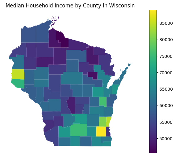
The returned object will be a GeoPandas GeoDataFrame, which can be used for mapping and spatial analysis. For example, you could create a simple choropleth map:
import matplotlib.pyplot as plt

# Plot the data (if using a Jupyter notebook, you might want to use %matplotlib inline)
fig, ax = plt.subplots(1, figsize=(10, 6))
wi_income_geo.plot(column='B19013_001E', cmap='viridis', legend=True, ax=ax)
ax.set_title('Median Household Income by County in Wisconsin')
plt.axis('off')
plt.show()
Debugging pytidycensus errors
At times, you may think that you’ve formatted your use of a pytidycensus function correctly but the Census API doesn’t return the data you expected. Whenever possible, pytidycensus carries through the error message from the Census API or translates common errors for the user.
To assist with debugging errors, or more generally to help users understand how pytidycensus functions are being translated to Census API calls, pytidycensus offers a parameter show_call that when set to True prints out the actual API call that pytidycensus is making to the Census API.
cbsa_bachelors = tc.get_acs(
    geography="cbsa",
    variables="DP02_0068P",
    year=2019,
    show_call=True
)
Getting data from the 2015-2019 5-year ACS
Mixed table types detected: ['DP', 'BC']. Making separate API calls.
Fetching 2 variables from DP tables
Census API call: https://api.census.gov/data/2019/acs/acs5/profile?get=DP02_0068PE%2CDP02_0068PM&key=983980b9fc504149e82117c949d7ed44653dc507&for=metropolitan+statistical+area%2Fmicropolitan+statistical+area%3A%2A
Fetching 1 variables from BC tables
Census API call: https://api.census.gov/data/2019/acs/acs5?get=NAME&key=983980b9fc504149e82117c949d7ed44653dc507&for=metropolitan+statistical+area%2Fmicropolitan+statistical+area%3A%2A
The printed URL can be copy-pasted into a web browser where users can see the raw JSON returned by the Census API and inspect the results.
Conclusion
This introduction to pytidycensus has covered the basics of retrieving and working with Census data in Python. The package provides a convenient interface to access data from the US Census Bureau’s APIs, with built-in support for spatial data analysis. For more information and examples, please refer to the examples directory and the package documentation.
Credits
Thannks to Kyle Walker for developing this amazing tutorial in R, which I ported to Python.