Basic usage of pytidycensus

This notebook demonstrates the basic functionality of pytidycensus, a Python library for accessing US Census Bureau data with pandas and GeoPandas support.

Setup

First, let’s install and import the necessary packages:

# Uncomment to install if running in Colab
# !pip install pytidycensus matplotlib

import pytidycensus as tc
import pandas as pd
import matplotlib.pyplot as plt
import seaborn as sns

# Set styling
plt.style.use('default')
sns.set_palette("husl")

Census API Key

To use pytidycensus, you need a free API key from the US Census Bureau. Get one at: https://api.census.gov/data/key_signup.html

Set your API key:

# Replace with your actual API key
tc.set_census_api_key("Your API Key Here")

# # Alternatively, set as environment variable:
# import os
# os.environ['CENSUS_API_KEY'] = 'Your API Key Here'

Ignore this cell. I am just loading my credentials from a yaml file in the parent directory.

import os
# Try to get API key from environment
api_key = os.environ.get("CENSUS_API_KEY")

# For documentation builds without a key, we'll mock the responses
try:
    tc.set_census_api_key(api_key)
    print("Using Census API key from environment")
except Exception:
    print("Using example API key for documentation")
    # This won't make real API calls during documentation builds
    tc.set_census_api_key("EXAMPLE_API_KEY_FOR_DOCS")

Census API key has been set for this session.
Using Census API key from environment

Core Functions

pytidycensus provides two main functions:

• get_decennial(): Access to 2000, 2010, and 2020 decennial US Census APIs

• get_acs(): Access to 1-year and 5-year American Community Survey APIs

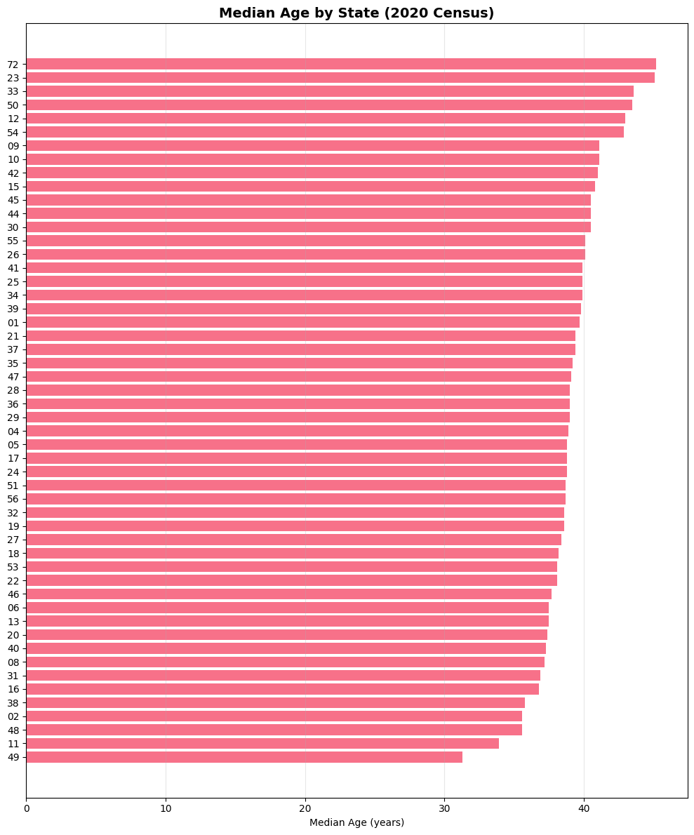
Example: Median Age by State (2020 Census)

Let’s look at median age by state from the 2020 Census:

# Get median age by state from 2020 Census
age_2020 = tc.get_decennial(
    geography="state",
    variables="P13_001N",  # Median age variable
    year=2020,
    sumfile="dhc"  # Demographic and Housing Characteristics file
)

print(f"Data shape: {age_2020.shape}")
age_2020.head()

Getting data from the 2020 decennial Census
Using the Demographic and Housing Characteristics File
Data shape: (52, 5)

/home/mmann1123/Documents/github/pytidycensus/pytidycensus/decennial.py:429: UserWarning: Note: 2020 decennial Census data use differential privacy, a technique that introduces errors into data to preserve respondent confidentiality. Small counts should be interpreted with caution. See https://www.census.gov/library/fact-sheets/2021/protecting-the-confidentiality-of-the-2020-census-redistricting-data.html for additional guidance.
  warnings.warn(

	state	GEOID	NAME	variable	estimate
0	09	09	Connecticut	P13_001N	41.1
1	10	10	Delaware	P13_001N	41.1
2	11	11	DC	P13_001N	33.9
3	12	12	Florida	P13_001N	43.0
4	13	13	Georgia	P13_001N	37.5

The function returns a pandas DataFrame with four columns:

• GEOID: Identifier for the geographical unit

• NAME: Descriptive name of the geographical unit

• variable: Census variable represented in the row

• value: Value of the variable for that unit

Visualizing the Data

Since we have a tidy DataFrame, we can easily visualize it:

# Create a horizontal bar plot
plt.figure(figsize=(10, 12))

# Sort by median age and plot
age_sorted = age_2020.sort_values('estimate', ascending=True).reset_index(drop=True)
plt.barh(range(len(age_sorted)), age_sorted['estimate'])
plt.yticks(range(len(age_sorted)), age_sorted['state'])
plt.xlabel('Median Age (years)')
plt.title('Median Age by State (2020 Census)', fontsize=14, fontweight='bold')
plt.grid(axis='x', alpha=0.3)
plt.tight_layout()
plt.show()

Geography in pytidycensus

pytidycensus supports many geographic levels. Here are the most commonly used:

Geography	Definition	Example Usage
"us"	United States	National data
"state"	State or equivalent	State-level data
"county"	County or equivalent	County-level data
"tract"	Census tract	Neighborhood-level data
"block group"	Census block group	Sub-neighborhood data
"place"	Census-designated place	City/town data
"zcta"	ZIP Code Tabulation Area	ZIP code areas

Example: County Data

Let’s get population data for counties in Texas:

# Get total population for Texas counties
tx_pop = tc.get_decennial(
    geography="county",
    variables="P1_001N",  # Total population
    state="TX",  # Filter to Texas
    year=2020
)

print(f"Number of Texas counties: {len(tx_pop)}")
tx_pop.head()

Getting data from the 2020 decennial Census
Using the PL 94-171 Redistricting Data Summary File
Number of Texas counties: 254

/home/mmann1123/Documents/github/pytidycensus/pytidycensus/decennial.py:429: UserWarning: Note: 2020 decennial Census data use differential privacy, a technique that introduces errors into data to preserve respondent confidentiality. Small counts should be interpreted with caution. See https://www.census.gov/library/fact-sheets/2021/protecting-the-confidentiality-of-the-2020-census-redistricting-data.html for additional guidance.
  warnings.warn(

	state	county	GEOID	NAME	variable	estimate
0	48	001	48001	Anderson County, Texas	P1_001N	57922
1	48	003	48003	Andrews County, Texas	P1_001N	18610
2	48	005	48005	Angelina County, Texas	P1_001N	86395
3	48	007	48007	Aransas County, Texas	P1_001N	23830
4	48	009	48009	Archer County, Texas	P1_001N	8560

Searching for Variables

The Census has thousands of variables. Use load_variables() to search for what you need:

# Load variables for 2022 5-year ACS
variables_2022 = tc.load_variables(2022, "acs", "acs5", cache=True)

print(f"Total variables available: {len(variables_2022)}")
variables_2022.head()

Loaded cached variables for 2022 acs acs5
Total variables available: 28193

	name	label	concept	predicateType	group	limit	table
0	AIANHH	Geography			N/A	0	NaN
1	AIHHTL	Geography			N/A	0	NaN
2	AIRES	Geography			N/A	0	NaN
3	ANRC	Geography			N/A	0	NaN
4	B01001A_001E	Estimate!!Total:	Sex by Age (White Alone)	int	B01001A	0	B01001A

# Search for income-related variables
income_vars = tc.search_variables("median household income", 2022, "acs", "acs5")
print(f"Found {len(income_vars)} income-related variables")
income_vars[['name', 'label']].head(10)

Loaded cached variables for 2022 acs acs5
Found 25 income-related variables

	name	label
0	B19013A_001E	Estimate!!Median household income in the past ...
1	B19013B_001E	Estimate!!Median household income in the past ...
2	B19013C_001E	Estimate!!Median household income in the past ...
3	B19013D_001E	Estimate!!Median household income in the past ...
4	B19013E_001E	Estimate!!Median household income in the past ...
5	B19013F_001E	Estimate!!Median household income in the past ...
6	B19013G_001E	Estimate!!Median household income in the past ...
7	B19013H_001E	Estimate!!Median household income in the past ...
8	B19013I_001E	Estimate!!Median household income in the past ...
9	B19013_001E	Estimate!!Median household income in the past ...

Working with ACS Data

American Community Survey (ACS) data includes estimates with margins of error, since it’s based on a sample rather than a complete count.

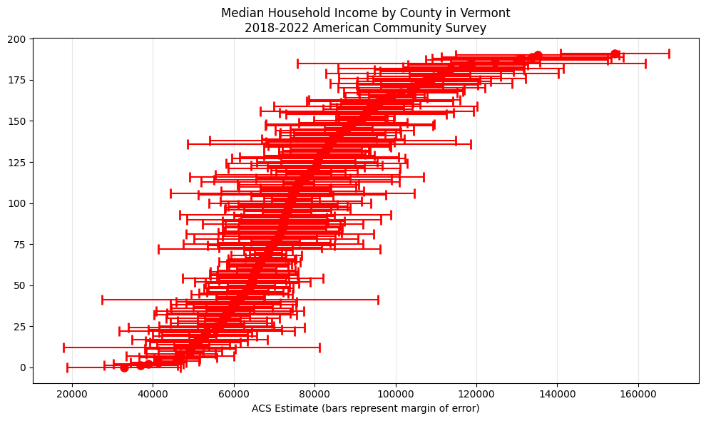
Example: Median Household Income

Let’s get median household income for Vermont counties:

# Get median household income for Vermont tracts
vt_income = tc.get_acs(
    geography="tract",
    variables={"medincome": "B19013_001"},  # Can use dictionary for variable names
    state="VT",
    year=2022,
    output="wide",  # Get data in wide format
)

vt_income

Getting data from the 2018-2022 5-year ACS

	GEOID	medincome	state	county	tract	NAME	medincome_moe
0	50001960100	96154	50	001	960100	Addison County, Vermont	18071.0
1	50001960200	106328	50	001	960200	Addison County, Vermont	22525.0
2	50001960300	72171	50	001	960300	Addison County, Vermont	19890.0
3	50001960400	99056	50	001	960400	Addison County, Vermont	5760.0
4	50001960500	75875	50	001	960500	Addison County, Vermont	15001.0
...	...	...	...	...	...	...	...
188	50027966501	64756	50	027	966501	Windsor County, Vermont	8833.0
189	50027966502	103750	50	027	966502	Windsor County, Vermont	12857.0
190	50027966600	64364	50	027	966600	Windsor County, Vermont	5805.0
191	50027966700	56875	50	027	966700	Windsor County, Vermont	12544.0
192	50027966800	68542	50	027	966800	Windsor County, Vermont	3365.0

193 rows × 7 columns

Notice that ACS data returns estimate and moe (margin of error) columns instead of a single value column.

Visualizing Uncertainty

We can visualize the uncertainty around estimates using error bars:

# Clean county names and create visualization
vt_clean = vt_income.copy()
vt_clean = vt_clean.sort_values("medincome")
vt_clean.dropna(subset=["medincome"], inplace=True)
plt.figure(figsize=(10, 6))

# Create error bar plot
plt.errorbar(
    vt_clean["medincome"],
    range(len(vt_clean)),
    xerr=vt_clean["medincome_moe"],  # Using margin of error as error bars
    fmt="o",
    color="red",
    markersize=8,
    capsize=5,
    capthick=2,
)

plt.xlabel('ACS Estimate (bars represent margin of error)')
plt.title('Median Household Income by County in Vermont\n2018-2022 American Community Survey')
plt.grid(axis='x', alpha=0.3)
plt.tight_layout()
plt.show()

Data Output Formats

By default, pytidycensus returns data in “tidy” format. You can also request “wide” format:

Tidy Format (Default)

# Multiple variables in tidy format
ca_demo_tidy = tc.get_acs(
    geography="county",
    variables={
        "total_pop": "B01003_001",
        "median_income": "B19013_001",
        "median_age": "B01002_001"
    },
    state="CA",
    year=2022,
    output="tidy"  # This is the default
)

print(f"Tidy format shape: {ca_demo_tidy.shape}")
ca_demo_tidy 

Getting data from the 2018-2022 5-year ACS
Tidy format shape: (174, 7)

	state	county	GEOID	NAME	variable	estimate	moe
0	06	001	06001	Alameda County, California	total_pop	1663823.0	NaN
1	06	003	06003	Alpine County, California	total_pop	1515.0	206.0
2	06	005	06005	Amador County, California	total_pop	40577.0	NaN
3	06	007	06007	Butte County, California	total_pop	213605.0	NaN
4	06	009	06009	Calaveras County, California	total_pop	45674.0	NaN
...	...	...	...	...	...	...	...
169	06	107	06107	Tulare County, California	median_age	31.5	0.2
170	06	109	06109	Tuolumne County, California	median_age	48.7	0.4
171	06	111	06111	Ventura County, California	median_age	39.0	0.2
172	06	113	06113	Yolo County, California	median_age	32.0	0.2
173	06	115	06115	Yuba County, California	median_age	33.5	0.3

174 rows × 7 columns

Wide Format

# Same data in wide format
ca_demo_wide = tc.get_acs(
    geography="county",
    variables={
        "total_pop": "B01003_001",
        "median_income": "B19013_001", 
        "median_age": "B01002_001"
    },
    state="CA",
    year=2022,
    output="wide"
)

print(f"Wide format shape: {ca_demo_wide.shape}")
ca_demo_wide.head()

Getting data from the 2018-2022 5-year ACS
Wide format shape: (58, 10)

	GEOID	total_pop	median_income	median_age	state	county	NAME	total_pop_moe	median_income_moe	median_age_moe
0	06001	1663823	122488	38.4	06	001	Alameda County, California	<NA>	1231.0	0.2
1	06003	1515	101125	43.0	06	003	Alpine County, California	206.0	17442.0	10.5
2	06005	40577	74853	49.6	06	005	Amador County, California	<NA>	6048.0	0.4
3	06007	213605	66085	36.5	06	007	Butte County, California	<NA>	2261.0	0.3
4	06009	45674	77526	52.1	06	009	Calaveras County, California	<NA>	3875.0	0.6

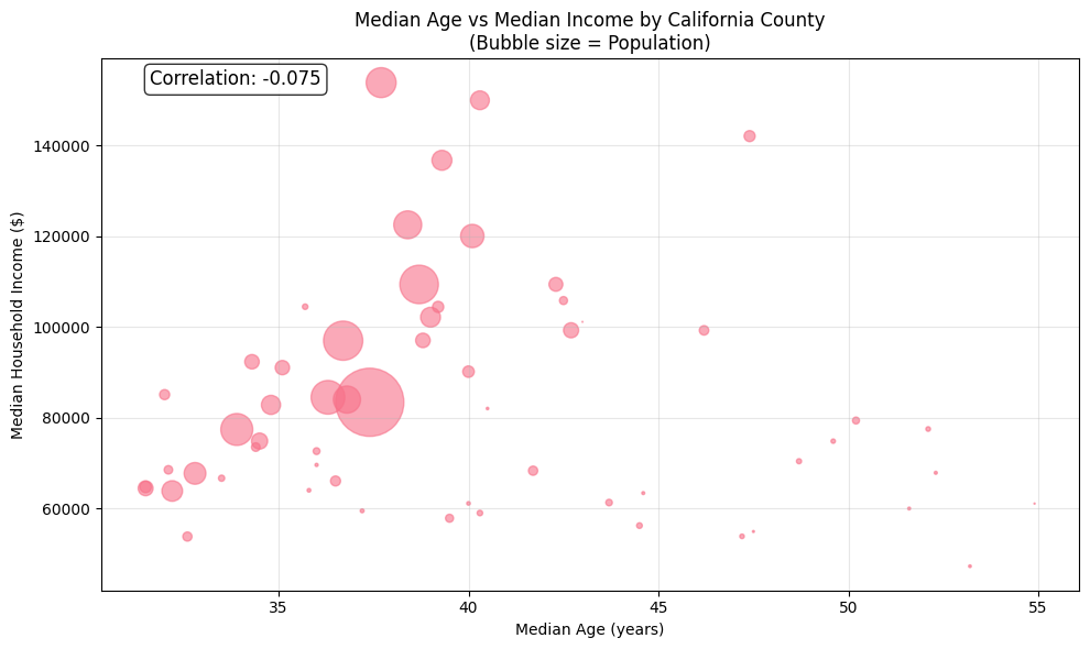
Multiple Variables Analysis

Let’s analyze the relationship between different demographic variables:

# Create scatter plot of median age vs median income
plt.figure(figsize=(10, 6))

plt.scatter(
    ca_demo_wide['median_age'], 
    ca_demo_wide['median_income'],
    s=ca_demo_wide['total_pop']/5000,  # Size by population
    alpha=0.6
)

plt.xlabel('Median Age (years)')
plt.ylabel('Median Household Income ($)')
plt.title('Median Age vs Median Income by California County\n(Bubble size = Population)')
plt.grid(alpha=0.3)

# Add correlation coefficient
correlation = ca_demo_wide['median_age'].corr(ca_demo_wide['median_income'])
plt.text(0.05, 0.95, f'Correlation: {correlation:.3f}', 
         transform=plt.gca().transAxes, fontsize=12,
         bbox=dict(boxstyle='round', facecolor='white', alpha=0.8))

plt.tight_layout()
plt.show()

Working with Different Survey Types

The ACS has different survey periods:

• 5-year ACS (survey="acs5"): More reliable for small areas, 5-year average

• 1-year ACS (survey="acs1"): More current, only for areas with 65,000+ population

# Compare 1-year vs 5-year estimates for large cities
cities_5yr = tc.get_acs(
    geography="place",
    variables="B19013_001",
    state="CA", 
    year=2022,
    survey="acs5"
)

cities_1yr = tc.get_acs(
    geography="place",
    variables="B19013_001",
    state="CA",
    year=2022, 
    survey="acs1"
)

print(f"5-year ACS places: {len(cities_5yr)}")
print(f"1-year ACS places: {len(cities_1yr)}")
print("\n1-year ACS is only available for larger places:")
cities_1yr.head()

Getting data from the 2018-2022 5-year ACS
Getting data from the 2022 1-year ACS
The 1-year ACS provides data for geographies with populations of 65,000 and greater.
5-year ACS places: 1611
1-year ACS places: 142

1-year ACS is only available for larger places:

	NAME	state	place	GEOID	variable	estimate	moe
0	Alameda city, California	06	00562	0600562	B19013_001	131116	11963.0
1	Alhambra city, California	06	00884	0600884	B19013_001	72406	11887.0
2	Anaheim city, California	06	02000	0602000	B19013_001	85133	4032.0
3	Antioch city, California	06	02252	0602252	B19013_001	100178	13978.0
4	Apple Valley town, California	06	02364	0602364	B19013_001	56187	7004.0

Summary

In this notebook, we learned:

1. Setup: How to install pytidycensus and set your API key

2. Core functions: get_decennial() and get_acs() for different data sources

3. Geographic levels: From national to neighborhood-level data

4. Variable search: Using load_variables() and search_variables()

5. Data formats: Tidy vs wide format output

6. Uncertainty: Working with ACS margins of error

7. Visualization: Creating plots with matplotlib

Next Steps

• Spatial Analysis: See 02_spatial_data.ipynb for mapping examples

• Advanced ACS: Explore 03_margins_of_error.ipynb for statistical techniques

• Other Datasets: Check 04_other_datasets.ipynb for population estimates

• Microdata: Learn about PUMS data in 05_pums_data.ipynb

Resources

• pytidycensus Documentation

• Census Variable Search

• Census Bureau Data