Simple Time Series Analysis with Census Data
This tutorial teaches you how to analyze changes in demographic data over time using the US Census Bureau’s datasets. We’ll focus on geographic levels that don’t change over time (like states and counties) to keep things simple and avoid complex boundary adjustments.
What You’ll Learn
The Golden Rule: Only compare like survey types (ACS5↔ACS5, Decennial↔Decennial)
Population trends using decennial census data (2010 vs 2020)
Income trends using ACS 5-year data (2012 vs 2020)
Best practices for temporal analysis
Visualization techniques for demographic change
Why This Matters
Understanding demographic change over time helps with:
Urban planning and policy decisions
Business location and market analysis
Research on social and economic trends
Grant writing and community development
Setup: Import Libraries and API Key
First, let’s import the libraries we need and set up our Census API key.
# Import required libraries
import pytidycensus as tc
import pandas as pd
import matplotlib.pyplot as plt
import numpy as np

# Make plots look nicer
plt.style.use('default')
plt.rcParams['figure.figsize'] = (12, 8)
plt.rcParams['font.size'] = 11

print("Libraries imported successfully!")
print(f"Using pytidycensus version: {tc.__version__}")
Libraries imported successfully!
Using pytidycensus version: 1.0.4
# Set your Census API key here
# Get a free key at: https://api.census.gov/data/key_signup.html

# UNCOMMENT and add your key:
# tc.set_census_api_key("YOUR_API_KEY_HERE")

print(" Remember to set your Census API key above!")
print("   Get one free at: https://api.census.gov/data/key_signup.html")
 Remember to set your Census API key above!
   Get one free at: https://api.census.gov/data/key_signup.html
The Golden Rule of Census Time Series
CRITICAL: Only compare surveys of the same type!
✅ CORRECT Comparisons
Decennial 2010 ↔ Decennial 2020: Complete population counts
ACS 5-year 2012 ↔ ACS 5-year 2020: Same methodology, sample size
ACS 1-year 2019 ↔ ACS 1-year 2021: Recent estimates for large areas
❌ WRONG Comparisons
ACS 1-year ↔ ACS 5-year: Different sample sizes and time periods
Decennial ↔ ACS: Different methodologies (complete count vs. sample)
Why This Matters
# Let's demonstrate why survey type matters
print("SURVEY TYPE COMPARISON:")
print("=" * 50)
print("DECENNIAL CENSUS:")
print("   • Complete count of all households")
print("   • Very low margin of error")
print("   • Every 10 years (2010, 2020, 2030...)")
print("   • Best for: Long-term trends, small areas")
print()
print("ACS 5-YEAR:")
print("   • Sample survey (~3.5M addresses/year)")
print("   • 5 years of data combined for stability")
print("   • Available for all geographies")
print("   • Best for: Small areas, stable trends")
print()
print("ACS 1-YEAR:")
print("   • Sample survey (~3.5M addresses/year)")
print("   • Single year of data")
print("   • Only areas with 65,000+ population")
print("   • Best for: Large areas, recent trends")
SURVEY TYPE COMPARISON:
==================================================
DECENNIAL CENSUS:
   • Complete count of all households
   • Very low margin of error
   • Every 10 years (2010, 2020, 2030...)
   • Best for: Long-term trends, small areas

ACS 5-YEAR:
   • Sample survey (~3.5M addresses/year)
   • 5 years of data combined for stability
   • Available for all geographies
   • Best for: Small areas, stable trends

ACS 1-YEAR:
   • Sample survey (~3.5M addresses/year)
   • Single year of data
   • Only areas with 65,000+ population
   • Best for: Large areas, recent trends
Part 1: Population Change Analysis (Decennial Census)
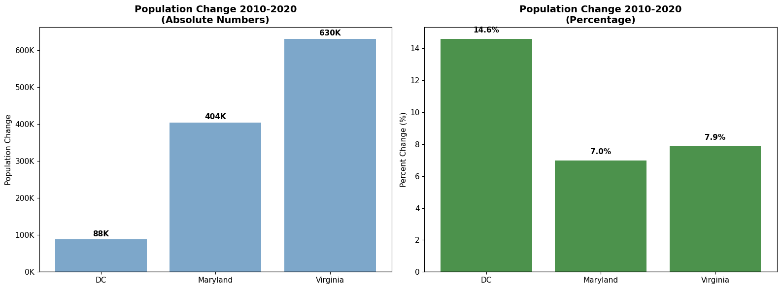
Let’s start by analyzing population changes in the Washington DC metro area between 2010 and 2020 using decennial census data. We’ll compare DC, Maryland, and Virginia at the state level.
Why Use State Level?
State boundaries don’t change over time
No need for complex boundary adjustments
Reliable and straightforward comparison
# Step 1: Get 2010 population data for DC metro states
print("   Fetching 2010 decennial census data...")
print("   Variable: P001001 (Total Population)")

# Define the states we want to analyze
metro_states = ["DC", "MD", "VA"]

# Get 2010 data
pop_2010 = tc.get_decennial(
    geography="state",
    variables={"total_pop": "P001001"},  # P001001 = Total Population in 2010
    state=metro_states,
    year=2010,
    output="wide"  # Wide format puts variables as columns
)

print(f"Retrieved data for {len(pop_2010)} states")
print("\n2010 Population Data:")
print(pop_2010[['NAME', 'total_pop']].to_string(index=False))
   Fetching 2010 decennial census data...
   Variable: P001001 (Total Population)
Getting data from the 2010 decennial Census
Using Census Summary File 1
Retrieved data for 3 states

2010 Population Data:
    NAME  total_pop
      DC     601723
Maryland    5773552
Virginia    8001024
# Step 2: Get 2020 population data
print("   Fetching 2020 decennial census data...")
print("   Variable: P1_001N (Total Population)")
print("   Note: Variable codes changed between 2010 and 2020!")

# Get 2020 data - NOTE: Different variable code!
pop_2020 = tc.get_decennial(
    geography="state",
    variables={"total_pop": "P1_001N"},  # P1_001N = Total Population in 2020
    state=metro_states,
    year=2020,
    output="wide"
)

print(f"Retrieved data for {len(pop_2020)} states")
print("\n2020 Population Data:")
print(pop_2020[['NAME', 'total_pop']].to_string(index=False))
   Fetching 2020 decennial census data...
   Variable: P1_001N (Total Population)
   Note: Variable codes changed between 2010 and 2020!
Getting data from the 2020 decennial Census
Using the PL 94-171 Redistricting Data Summary File
Retrieved data for 3 states

2020 Population Data:
    NAME  total_pop
      DC     689545
Maryland    6177224
Virginia    8631393
/home/mmann1123/Documents/github/pytidycensus/pytidycensus/decennial.py:429: UserWarning: Note: 2020 decennial Census data use differential privacy, a technique that introduces errors into data to preserve respondent confidentiality. Small counts should be interpreted with caution. See https://www.census.gov/library/fact-sheets/2021/protecting-the-confidentiality-of-the-2020-census-redistricting-data.html for additional guidance.
  warnings.warn(
🔍 Key Learning Point: Variable Codes Change!
Notice that we used different variable codes:
2010:
P0010012020:
P1_001N
This is common when comparing across census years. Always check variable definitions!
# Step 3: Merge the data and calculate changes
print("   Calculating population changes...")

# Merge 2010 and 2020 data on state name
pop_change = pd.merge(
    pop_2010[['NAME', 'total_pop']].rename(columns={'total_pop': 'pop_2010'}),
    pop_2020[['NAME', 'total_pop']].rename(columns={'total_pop': 'pop_2020'}),
    on='NAME'
)

# Calculate absolute and percentage changes
pop_change['change_absolute'] = pop_change['pop_2020'] - pop_change['pop_2010']
pop_change['change_percent'] = (pop_change['change_absolute'] / pop_change['pop_2010']) * 100

print("Population change analysis complete!")
print("\nPopulation Change Summary (2010-2020):")
print("=" * 60)

for _, row in pop_change.iterrows():
    print(f"{row['NAME']}:")
    print(f"   2010: {row['pop_2010']:,}")
    print(f"   2020: {row['pop_2020']:,}")
    print(f"   Change: {row['change_absolute']:+,} ({row['change_percent']:+.1f}%)")
    print()
   Calculating population changes...
Population change analysis complete!

Population Change Summary (2010-2020):
============================================================
DC:
   2010: 601,723
   2020: 689,545
   Change: +87,822 (+14.6%)

Maryland:
   2010: 5,773,552
   2020: 6,177,224
   Change: +403,672 (+7.0%)

Virginia:
   2010: 8,001,024
   2020: 8,631,393
   Change: +630,369 (+7.9%)
# Step 4: Visualize the population changes
fig, (ax1, ax2) = plt.subplots(1, 2, figsize=(16, 6))

# Chart 1: Absolute change
colors = ['red' if x < 0 else 'steelblue' for x in pop_change['change_absolute']]
bars1 = ax1.bar(pop_change['NAME'], pop_change['change_absolute'], color=colors, alpha=0.7)
ax1.set_title('Population Change 2010-2020\n(Absolute Numbers)', fontsize=14, fontweight='bold')
ax1.set_ylabel('Population Change')
ax1.axhline(y=0, color='black', linestyle='-', alpha=0.3)
ax1.yaxis.set_major_formatter(plt.FuncFormatter(lambda x, p: f'{x/1000:.0f}K'))

# Add value labels on bars
for bar, value in zip(bars1, pop_change['change_absolute']):
    height = bar.get_height()
    ax1.text(bar.get_x() + bar.get_width()/2., height + (5000 if height >= 0 else -15000),
             f'{value/1000:.0f}K', ha='center', va='bottom' if height >= 0 else 'top', fontweight='bold')

# Chart 2: Percentage change
colors2 = ['red' if x < 0 else 'darkgreen' for x in pop_change['change_percent']]
bars2 = ax2.bar(pop_change['NAME'], pop_change['change_percent'], color=colors2, alpha=0.7)
ax2.set_title('Population Change 2010-2020\n(Percentage)', fontsize=14, fontweight='bold')
ax2.set_ylabel('Percent Change (%)')
ax2.axhline(y=0, color='black', linestyle='-', alpha=0.3)

# Add value labels on bars
for bar, value in zip(bars2, pop_change['change_percent']):
    height = bar.get_height()
    ax2.text(bar.get_x() + bar.get_width()/2., height + (0.3 if height >= 0 else -0.8),
             f'{value:.1f}%', ha='center', va='bottom' if height >= 0 else 'top', fontweight='bold')

plt.tight_layout()
plt.show()

# Summary statistics
total_2010 = pop_change['pop_2010'].sum()
total_2020 = pop_change['pop_2020'].sum()
total_change = total_2020 - total_2010
total_pct = (total_change / total_2010) * 100

print(f"DC METRO AREA SUMMARY:")
print(f"   Total 2010 Population: {total_2010:,}")
print(f"   Total 2020 Population: {total_2020:,}")
print(f"   Net Change: {total_change:+,} ({total_pct:+.1f}%)")
DC METRO AREA SUMMARY:
   Total 2010 Population: 14,376,299
   Total 2020 Population: 15,498,162
   Net Change: +1,121,863 (+7.8%)
Part 2: Income Change Analysis (ACS 5-Year Data)
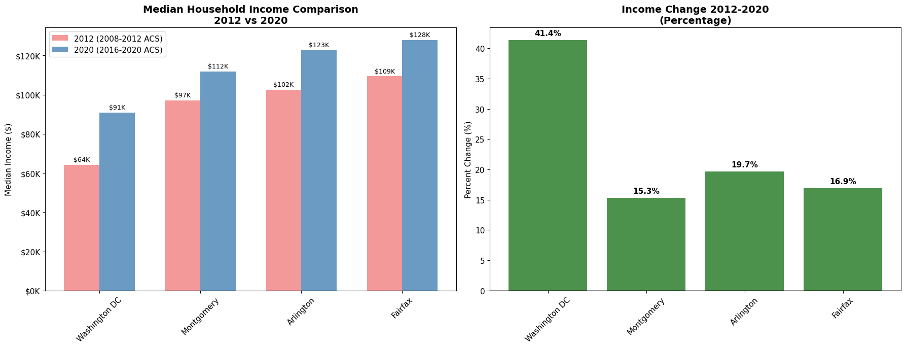
Now let’s analyze how median household income changed in the DC metro area using ACS 5-year data. We’ll compare 2012 (2008-2012 ACS) with 2020 (2016-2020 ACS).
Why These Years?
2012 ACS 5-year: Represents 2008-2012 period (pre-recession recovery)
2020 ACS 5-year: Represents 2016-2020 period (recent data)
8-year gap: Provides meaningful temporal separation
County-Level Analysis
We’ll look at specific counties in the DC metro area that are economically important.
# Define the counties we want to analyze
counties_to_analyze = [
    {"state": "DC", "county": None, "display_name": "Washington DC"},
    {"state": "MD", "county": "Montgomery County", "display_name": "Montgomery County, MD"},
    {"state": "VA", "county": "Arlington County", "display_name": "Arlington County, VA"},
    {"state": "VA", "county": "Fairfax County", "display_name": "Fairfax County, VA"}
]

print("Target Counties for Income Analysis:")
for county in counties_to_analyze:
    print(f"   • {county['display_name']}")
print()
print("Variable: B19013_001E (Median Household Income)")
print("Comparing: 2012 ACS 5-year vs 2020 ACS 5-year")
Target Counties for Income Analysis:
   • Washington DC
   • Montgomery County, MD
   • Arlington County, VA
   • Fairfax County, VA

Variable: B19013_001E (Median Household Income)
Comparing: 2012 ACS 5-year vs 2020 ACS 5-year
# Step 1: Get 2012 ACS income data
print("Fetching 2012 ACS 5-year data (2008-2012)...")

income_2012_data = []

for county_info in counties_to_analyze:
    try:
        income_data = tc.get_acs(
            geography="county",
            variables={"median_income": "B19013_001E"},
            state=county_info["state"],
            county=county_info["county"],  # None for DC (state-equivalent)
            year=2012,
            survey="acs5",
            output="wide"
        )

        # Add display name for easier tracking
        income_data['display_name'] = county_info['display_name']
        income_2012_data.append(income_data)

        print(f"    {county_info['display_name']}: ${income_data.iloc[0]['median_income']:,}")

    except Exception as e:
        print(f"    {county_info['display_name']}: Error - {str(e)[:50]}...")

# Combine all 2012 data
if income_2012_data:
    income_2012_combined = pd.concat(income_2012_data, ignore_index=True)
    print(f"\n Successfully retrieved 2012 data for {len(income_2012_combined)} counties")
else:
    print("\n  No 2012 data retrieved")
Fetching 2012 ACS 5-year data (2008-2012)...
Getting data from the 2008-2012 5-year ACS
    Washington DC: $64,267
Getting data from the 2008-2012 5-year ACS
    Montgomery County, MD: $96,985
Getting data from the 2008-2012 5-year ACS
    Arlington County, VA: $102,459
Getting data from the 2008-2012 5-year ACS
    Fairfax County, VA: $109,383

 Successfully retrieved 2012 data for 4 counties
# Step 2: Get 2020 ACS income data
print("Fetching 2020 ACS 5-year data (2016-2020)...")

income_2020_data = []

for county_info in counties_to_analyze:
    try:
        income_data = tc.get_acs(
            geography="county",
            variables={"median_income": "B19013_001E"},
            state=county_info["state"],
            county=county_info["county"],
            year=2020,
            survey="acs5",
            output="wide"
        )

        income_data['display_name'] = county_info['display_name']
        income_2020_data.append(income_data)

        print(f"    {county_info['display_name']}: ${income_data.iloc[0]['median_income']:,}")

    except Exception as e:
        print(f"    {county_info['display_name']}: Error - {str(e)[:50]}...")

# Combine all 2020 data
if income_2020_data:
    income_2020_combined = pd.concat(income_2020_data, ignore_index=True)
    print(f"\n Successfully retrieved 2020 data for {len(income_2020_combined)} counties")
else:
    print("\n No 2020 data retrieved")
Fetching 2020 ACS 5-year data (2016-2020)...
Getting data from the 2016-2020 5-year ACS
    Washington DC: $90,842
Getting data from the 2016-2020 5-year ACS
    Montgomery County, MD: $111,812
Getting data from the 2016-2020 5-year ACS
    Arlington County, VA: $122,604
Getting data from the 2016-2020 5-year ACS
    Fairfax County, VA: $127,866

 Successfully retrieved 2020 data for 4 counties
# Step 3: Calculate income changes
if 'income_2012_combined' in locals() and 'income_2020_combined' in locals():
    print("   Calculating income changes...")

    # Merge data on display name
    income_change = pd.merge(
        income_2012_combined[['display_name', 'median_income']].rename(columns={'median_income': 'income_2012'}),
        income_2020_combined[['display_name', 'median_income']].rename(columns={'median_income': 'income_2020'}),
        on='display_name'
    )

    # Calculate changes
    income_change['change_absolute'] = income_change['income_2020'] - income_change['income_2012']
    income_change['change_percent'] = (income_change['change_absolute'] / income_change['income_2012']) * 100

    print(" Income change analysis complete!")
    print("\nMedian Income Change Summary (2012-2020):")
    print("=" * 70)

    for _, row in income_change.iterrows():
        print(f" {row['display_name']}:")
        print(f"   2012: ${row['income_2012']:,}")
        print(f"   2020: ${row['income_2020']:,}")
        print(f"   Change: ${row['change_absolute']:+,} ({row['change_percent']:+.1f}%)")
        print()
else:
    print("Cannot calculate changes - missing data")
    income_change = pd.DataFrame()  # Empty dataframe for later checks
   Calculating income changes...
 Income change analysis complete!

Median Income Change Summary (2012-2020):
======================================================================
 Washington DC:
   2012: $64,267
   2020: $90,842
   Change: $+26,575 (+41.4%)

 Montgomery County, MD:
   2012: $96,985
   2020: $111,812
   Change: $+14,827 (+15.3%)

 Arlington County, VA:
   2012: $102,459
   2020: $122,604
   Change: $+20,145 (+19.7%)

 Fairfax County, VA:
   2012: $109,383
   2020: $127,866
   Change: $+18,483 (+16.9%)
# Step 4: Visualize income changes
if not income_change.empty:
    fig, (ax1, ax2) = plt.subplots(1, 2, figsize=(18, 7))

    # Chart 1: Income levels comparison
    x = np.arange(len(income_change))
    width = 0.35

    bars1 = ax1.bar(x - width/2, income_change['income_2012'], width,
                    label='2012 (2008-2012 ACS)', color='lightcoral', alpha=0.8)
    bars2 = ax1.bar(x + width/2, income_change['income_2020'], width,
                    label='2020 (2016-2020 ACS)', color='steelblue', alpha=0.8)

    ax1.set_title('Median Household Income Comparison\n2012 vs 2020', fontsize=14, fontweight='bold')
    ax1.set_ylabel('Median Income ($)')
    ax1.set_xticks(x)
    ax1.set_xticklabels([name.replace(' County', '').replace(', VA', '').replace(', MD', '')
                        for name in income_change['display_name']], rotation=45)
    ax1.legend()
    ax1.yaxis.set_major_formatter(plt.FuncFormatter(lambda x, p: f'${x/1000:.0f}K'))

    # Add value labels
    for bar in bars1:
        height = bar.get_height()
        ax1.text(bar.get_x() + bar.get_width()/2., height + 1000,
                f'${height/1000:.0f}K', ha='center', va='bottom', fontsize=9)

    for bar in bars2:
        height = bar.get_height()
        ax1.text(bar.get_x() + bar.get_width()/2., height + 1000,
                f'${height/1000:.0f}K', ha='center', va='bottom', fontsize=9)

    # Chart 2: Percentage change
    colors = ['red' if x < 0 else 'darkgreen' for x in income_change['change_percent']]
    bars3 = ax2.bar(income_change['display_name'].str.replace(' County', '').str.replace(', VA', '').str.replace(', MD', ''),
                    income_change['change_percent'], color=colors, alpha=0.7)

    ax2.set_title('Income Change 2012-2020\n(Percentage)', fontsize=14, fontweight='bold')
    ax2.set_ylabel('Percent Change (%)')
    ax2.axhline(y=0, color='black', linestyle='-', alpha=0.3)
    ax2.tick_params(axis='x', rotation=45)

    # Add value labels
    for bar, value in zip(bars3, income_change['change_percent']):
        height = bar.get_height()
        ax2.text(bar.get_x() + bar.get_width()/2., height + (0.5 if height >= 0 else -1.5),
                f'{value:.1f}%', ha='center', va='bottom' if height >= 0 else 'top', fontweight='bold')

    plt.tight_layout()
    plt.show()

    # Summary statistics
    avg_change = income_change['change_percent'].mean()
    print(f"INCOME ANALYSIS SUMMARY:")
    print(f"   Average income change: {avg_change:.1f}%")
    print(f"   Counties with income growth: {(income_change['change_percent'] > 0).sum()}")
    print(f"   Counties with income decline: {(income_change['change_percent'] < 0).sum()}")

else:
    print("   Cannot create visualization - no income data available")
    print("   This might be due to API key issues or data availability")
INCOME ANALYSIS SUMMARY:
   Average income change: 23.3%
   Counties with income growth: 4
   Counties with income decline: 0
Part 3: Understanding Your Results
What Do These Numbers Mean?
Population Changes (Decennial Census)
Shows actual population growth or decline
DC typically shows high growth due to urban revitalization
Suburban areas may show different patterns
Income Changes (ACS 5-Year)
Reflects economic conditions over time
Adjusted for inflation, this shows real purchasing power changes
High-income areas often show faster income growth
Important Considerations
# Let's discuss data quality and limitations
print("  IMPORTANT DATA QUALITY CONSIDERATIONS:")
print("=" * 50)
print()
print(" DECENNIAL CENSUS:")
print("    Advantages:")
print("      • Complete population count (not a sample)")
print("      • Very accurate for population totals")
print("      • Available for all geographic levels")
print("    Limitations:")
print("      • Only every 10 years")
print("      • Limited variables (basic demographics only)")
print("      • 2020 data uses differential privacy (slight noise added)")
print()
print(" ACS 5-YEAR:")
print("    Advantages:")
print("      • Rich set of variables (income, education, housing, etc.)")
print("      • Annual updates")
print("      • Available for small geographies")
print("    Limitations:")
print("      • Sample-based (margins of error)")
print("      • 5-year averages may mask recent changes")
print("      • Smaller areas have larger margins of error")
print()
print(" BEST PRACTICES:")
print("   • Always check margins of error for ACS data")
print("   • Consider real vs. nominal changes (adjust for inflation)")
print("   • Look for consistent patterns across multiple indicators")
print("   • Document your methodology and assumptions")
  IMPORTANT DATA QUALITY CONSIDERATIONS:
==================================================

 DECENNIAL CENSUS:
    Advantages:
      • Complete population count (not a sample)
      • Very accurate for population totals
      • Available for all geographic levels
    Limitations:
      • Only every 10 years
      • Limited variables (basic demographics only)
      • 2020 data uses differential privacy (slight noise added)

 ACS 5-YEAR:
    Advantages:
      • Rich set of variables (income, education, housing, etc.)
      • Annual updates
      • Available for small geographies
    Limitations:
      • Sample-based (margins of error)
      • 5-year averages may mask recent changes
      • Smaller areas have larger margins of error

 BEST PRACTICES:
   • Always check margins of error for ACS data
   • Consider real vs. nominal changes (adjust for inflation)
   • Look for consistent patterns across multiple indicators
   • Document your methodology and assumptions
Part 4: Advanced Topics and Next Steps
When Geographic Boundaries Change
For this tutorial, we used states and counties because their boundaries are stable over time. But what if you need to analyze census tracts or other small geographies that change?
Solution: Area Interpolation
Use the
toblerlibrary’sarea_interpolate()functionRedistributes data from old boundaries to new boundaries
Accounts for how areas were split or merged
See our advanced tutorial: time_series_analysis.md for tract-level analysis with boundary changes.
Summary: Key Takeaways
What You’ve Learned
The Golden Rule: Only compare like survey types
Decennial ↔ Decennial for population counts
ACS 5-year ↔ ACS 5-year for detailed demographics
Geographic Strategy: Use stable boundaries when possible
States and counties don’t change over time
Avoids complex boundary adjustments
Variable Consistency: Check codes across years
2010:
P001001vs 2020:P1_001Nfor populationACS variables are generally more consistent
Data Quality: Understand limitations
Decennial = complete count, ACS = sample
Check margins of error for ACS data
Consider real vs. nominal changes
Practical Applications
Urban Planning: Population growth patterns
Economic Development: Income trend analysis
Policy Research: Demographic change impacts
Business Analysis: Market area dynamics
Your Assignment
Try this analysis with your own area of interest:
Pick 3-4 states or counties
Run the population change analysis
Add income or another ACS variable
Create your own visualizations
Write a brief interpretation of the results
Happy analyzing!