Other Census Bureau datasets

Population Estimates Program (PEP)

• Purpose: Provides annual population estimates between decennial censuses

• Frequency: Updated annually

• Geographic Coverage: US, regions, divisions, states, counties, metro areas, places

• Time Range: 2010-present (function supports 2015+)

Specific Datasets Within PEP

1. Population Totals (product="population") - Basic population counts by geography - Annual estimates for intercensal years

2. Components of Change (product="components") - Births, deaths, migration flows - Natural change calculations - Domestic and international migration

3. Population Characteristics (product="characteristics") - Demographics by Age, Sex, Race, Hispanic Origin (ASRH) - Population breakdowns by key demographic categories

Key Parameters

• product: “population”, “components”, “characteristics”

• variables: “POP”, “BIRTHS”, “DEATHS”, migration variables, rates

• breakdown: [“SEX”, “RACE”, “ORIGIN”, “AGEGROUP”] for demographics

• vintage: Dataset version (e.g., 2024 for most recent)

• year: Specific data year (defaults to vintage)

• time_series: Get multi-year data

• geometry: Add geographic boundaries

• output: “tidy” (default) or “wide” format

Data Sources

• 2020+: CSV files from Census Bureau FTP servers

• 2015-2019: Census API (requires API key)

• Automatic handling: No user intervention needed

Geographic Support

All major Census geographies: US, regions, divisions, states, counties, CBSAs, CSAs, places

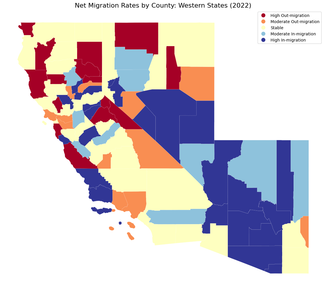
Mapping Migration Estimates

Let’s create a map of net migration rates:

Census API Key

To use pytidycensus, you need a free API key from the US Census Bureau. Get one at: https://api.census.gov/data/key_signup.html

import pytidycensus as tc
import pandas as pd
import matplotlib.pyplot as plt

tc.set_census_api_key("YOUR API KEY GOES HERE")

Ignore the next cell. It is just to show how users can load their credentials using the new utility function.

import os

# Try to get API key from environment
api_key = os.environ.get("CENSUS_API_KEY")

try:
    tc.set_census_api_key(api_key)
    print("Using Census API key from environment")
except Exception:
    print("Using example API key for documentation")
    tc.set_census_api_key("EXAMPLE_API_KEY_FOR_DOCS")

Census API key has been set for this session.
Using Census API key from environment

Product Types and Variables

The get_estimates() function supports three main products:

1. population (default) - Basic population totals

2. components - Components of population change

3. characteristics - Population by demographics

Available Variables

Common variables include:

• POP: Total population

• BIRTHS: Births

• DEATHS: Deaths

• DOMESTICMIG: Domestic migration

• INTERNATIONALMIG: International migration

• NETMIG: Net migration

• NATURALCHG: Natural change (births - deaths)

• RNETMIG: Net migration rate

#Get county data with geometry for mapping
counties_geo = tc.get_estimates(
    geography="county",
    variables="RNETMIG",  # Net migration rate
    year=2022,
    geometry=True,  # Include geometry for mapping
    state=["CA", "NV", "AZ"],  # Western states
)

print("County data with geometry:", counties_geo.shape)
print("Data types:", type(counties_geo))
counties_geo.head(3)

Getting data from the 2024 Population Estimates Program (vintage 2024)

/home/mmann1123/Documents/github/pytidycensus/pytidycensus/estimates.py:728: UserWarning: Using vintage 2024 data for year 2022. Consider setting vintage=2022 if available.
  warnings.warn(

Warning: Multiple states specified, will filter after download
Loading county boundaries...
County data with geometry: (90, 8)
Data types: <class 'geopandas.geodataframe.GeoDataFrame'>

	GEOID	NAME_x	geometry	STATEFP	COUNTYFP	NAMELSAD	NAME_y	RNETMIG2022
0	06091	Sierra	POLYGON ((-120.55587 39.50874, -120.55614 39.5...	06	091	Sierra County	Sierra County, California	-19.960080
1	32001	Churchill	POLYGON ((-119.22613 39.90038, -119.2261 39.90...	32	001	Churchill County	Churchill County, Nevada	9.048192
2	32013	Humboldt	POLYGON ((-119.33142 41.0391, -119.3314 41.041...	32	013	Humboldt County	Humboldt County, Nevada	-20.804677

Mapping with Geometry

Because we set geometry=True, the returned GeoDataFrame includes geometry data for mapping.

#Create a map of net migration rates
fig, ax = plt.subplots(figsize=(15, 10))

# Create migration categories for better visualization
counties_geo["migration_category"] = pd.cut(
    counties_geo["RNETMIG2022"],
    bins=[-float("inf"), -10, -5, 5, 10, float("inf")],
    labels=[
        "High Out-migration",
        "Moderate Out-migration",
        "Stable",
        "Moderate In-migration",
        "High In-migration",
    ],
)

# Plot the map
counties_geo.plot(
    column="migration_category",
    legend=True,
    ax=ax,
    cmap="RdYlBu",
    edgecolor="white",
    linewidth=0.1,
)

ax.set_title("Net Migration Rates by County: Western States (2022)", fontsize=16)
ax.set_axis_off()
plt.tight_layout()
plt.show()

Geographic Levels

Population estimates support multiple geographic levels beyond states:

# Metropolitan areas (CBSAs) 
metros = tc.get_estimates(
    geography="cbsa",
    variables="POP", 
    year=2022
)

print(f"Metro areas: {metros.shape[0]} CBSAs")
print("Largest metropolitan areas:")
metros_largest = metros.nlargest(10, 'POPESTIMATE2022')
print(metros_largest[['NAME', 'POPESTIMATE2022']])

/home/mmann1123/Documents/github/pytidycensus/pytidycensus/estimates.py:728: UserWarning: Using vintage 2024 data for year 2022. Consider setting vintage=2022 if available.
  warnings.warn(

Getting data from the 2024 Population Estimates Program (vintage 2024)
Metro areas: 925 CBSAs
Largest metropolitan areas:
                                              NAME  POPESTIMATE2022
1030            New York-Newark-Jersey City, NY-NJ         19619844
860             Los Angeles-Long Beach-Anaheim, CA         12906936
293                Chicago-Naperville-Elgin, IL-IN          9310017
394                Dallas-Fort Worth-Arlington, TX          7973603
640             Houston-Pasadena-The Woodlands, TX          7403068
1521  Washington-Arlington-Alexandria, DC-VA-MD-WV          6289810
65               Atlanta-Sandy Springs-Roswell, GA          6253070
1126   Philadelphia-Camden-Wilmington, PA-NJ-DE-MD          6252024
929      Miami-Fort Lauderdale-West Palm Beach, FL          6211194
1142                     Phoenix-Mesa-Chandler, AZ          5029933

# County-level data for Texas
tx_counties = tc.get_estimates(
    geography="county",
    variables="POP",
    state="TX",
    year=2022
)

print(f"Texas counties: {tx_counties.shape[0]} counties")
print("Largest Texas counties by population:")
tx_largest = tx_counties.nlargest(10, 'POPESTIMATE2022')
print(tx_largest[['NAME', 'POPESTIMATE2022']])

Getting data from the 2024 Population Estimates Program (vintage 2024)

/home/mmann1123/Documents/github/pytidycensus/pytidycensus/estimates.py:728: UserWarning: Using vintage 2024 data for year 2022. Consider setting vintage=2022 if available.
  warnings.warn(

Texas counties: 254 counties
Largest Texas counties by population:
                         NAME  POPESTIMATE2022
2669     Harris County, Texas          4806747
2625     Dallas County, Texas          2613712
2788    Tarrant County, Texas          2161670
2583      Bexar County, Texas          2063840
2795     Travis County, Texas          1332544
2611     Collin County, Texas          1163724
2629     Denton County, Texas           980355
2647  Fort Bend County, Texas           893319
2676    Hidalgo County, Texas           889799
2639    El Paso County, Texas           868890

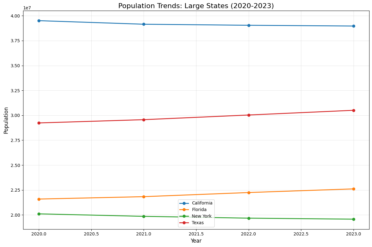
# Get time series data for select states
time_series_states = tc.get_estimates(
    geography="state",
    variables="POP",
    time_series=True,
    vintage=2023,  # Use 2023 vintage for data through 2023
    state=["CA", "TX", "FL", "NY"],  #Focus on large states
)

print("Time series data shape:", time_series_states.shape)
print("Years available:", sorted(time_series_states["year"].unique()))
time_series_states.head(10)

Getting data from the 2023 Population Estimates Program (vintage 2023)
Time series data shape: (16, 5)
Years available: [2020, 2021, 2022, 2023]

	GEOID	NAME	variable	year	estimate
0	06	California	POPESTIMATE	2020	39503200
1	12	Florida	POPESTIMATE	2020	21591299
2	36	New York	POPESTIMATE	2020	20104710
3	48	Texas	POPESTIMATE	2020	29234361
4	06	California	POPESTIMATE	2021	39145060
5	12	Florida	POPESTIMATE	2021	21830708
6	36	New York	POPESTIMATE	2021	19854526
7	48	Texas	POPESTIMATE	2021	29561286
8	06	California	POPESTIMATE	2022	39040616
9	12	Florida	POPESTIMATE	2022	22245521

# Plot population trends
plt.figure(figsize=(12, 8))

for state in time_series_states['NAME'].unique():
    state_data = time_series_states[time_series_states['NAME'] == state]
    plt.plot(state_data['year'], state_data['estimate'], 
             marker='o', linewidth=2, label=state)

plt.title('Population Trends: Large States (2020-2023)', fontsize=16)
plt.xlabel('Year', fontsize=12)
plt.ylabel('Population', fontsize=12)
plt.legend()
plt.grid(True, alpha=0.3)
plt.tight_layout()
plt.show()

Basic Population Estimates

Let’s start with basic population estimates by state:

# Get population estimates for US states
us_pop_estimates = tc.get_estimates(
    geography="state",
    variables="POP",
    year=2022
)

print(f"Shape: {us_pop_estimates.shape}")
print("Data format:", us_pop_estimates.columns.tolist())
us_pop_estimates.head()

Getting data from the 2024 Population Estimates Program (vintage 2024)
Shape: (52, 3)
Data format: ['GEOID', 'NAME', 'POPESTIMATE2022']

/home/mmann1123/Documents/github/pytidycensus/pytidycensus/estimates.py:728: UserWarning: Using vintage 2024 data for year 2022. Consider setting vintage=2022 if available.
  warnings.warn(

	GEOID	NAME	POPESTIMATE2022
14	01	Alabama	5076181
15	02	Alaska	734442
16	04	Arizona	7377566
17	05	Arkansas	3047704
18	06	California	39142414

# Get components of population change
us_components = tc.get_estimates(
    geography="state",
    product="components",  # Specify components product
    variables=["BIRTHS", "DEATHS", "DOMESTICMIG", "INTERNATIONALMIG"],
    year=2022,
    output="tidy"  # Tidy format for easier analysis
)

print("Components data shape:", us_components.shape)
print("Variables available:", us_components['variable'].unique())
us_components.head(10)

/home/mmann1123/Documents/github/pytidycensus/pytidycensus/estimates.py:728: UserWarning: Using vintage 2024 data for year 2022. Consider setting vintage=2022 if available.
  warnings.warn(

Getting data from the 2024 Population Estimates Program (vintage 2024)

Components data shape: (208, 4)
Variables available: ['BIRTHS2022' 'DEATHS2022' 'DOMESTICMIG2022' 'INTERNATIONALMIG2022']

	GEOID	NAME	variable	estimate
0	01	Alabama	BIRTHS2022	58103
1	02	Alaska	BIRTHS2022	9359
2	04	Arizona	BIRTHS2022	79173
3	05	Arkansas	BIRTHS2022	36115
4	06	California	BIRTHS2022	424071
5	08	Colorado	BIRTHS2022	62659
6	09	Connecticut	BIRTHS2022	35637
7	10	Delaware	BIRTHS2022	10849
8	11	District of Columbia	BIRTHS2022	8502
9	12	Florida	BIRTHS2022	221941

Demographic Breakdowns

One of the most powerful features is demographic breakdowns using the breakdown parameter. This accesses the Age, Sex, Race, Hispanic Origin (ASRH) datasets:

# Get population by sex for all states
pop_by_sex = tc.get_estimates(
    geography="state",
    variables="POP",
    breakdown=["SEX"],
    breakdown_labels=True, # Include human-readable labels
    year=2022
)

print("Population by sex data:")
print(pop_by_sex.head(10))

# Check the breakdown categories
if 'SEX_label' in pop_by_sex.columns:
    print("\nSex categories:", pop_by_sex['SEX_label'].unique())

Getting data from the 2024 Population Estimates Program (vintage 2024)

/home/mmann1123/Documents/github/pytidycensus/pytidycensus/estimates.py:728: UserWarning: Using vintage 2024 data for year 2022. Consider setting vintage=2022 if available.
  warnings.warn(

Processing characteristics data with breakdown: ['SEX']
Population by sex data:
   STATE        NAME  SEX  ORIGIN  RACE  AGE GEOID  estimate  year variable  \
0      1     Alabama    1       0     0    0    01     29531  2022      POP   
1      1     Alabama    2       0     0    0    01     28195  2022      POP   
2      2      Alaska    1       0     0    0    02      4808  2022      POP   
3      2      Alaska    2       0     0    0    02      4504  2022      POP   
4      4     Arizona    1       0     0    0    04     40228  2022      POP   
5      4     Arizona    2       0     0    0    04     38496  2022      POP   
6      5    Arkansas    1       0     0    0    05     18258  2022      POP   
7      5    Arkansas    2       0     0    0    05     17590  2022      POP   
8      6  California    1       0     0    0    06    217463  2022      POP   
9      6  California    2       0     0    0    06    208334  2022      POP   

  SEX_label  
0      Male  
1    Female  
2      Male  
3    Female  
4      Male  
5    Female  
6      Male  
7    Female  
8      Male  
9    Female  

Sex categories: ['Male' 'Female']