Margins of error in the ACS

Understanding and working with uncertainty in American Community Survey data.

import pytidycensus as tc
import pandas as pd
import numpy as np
import matplotlib.pyplot as plt

Census API Key

To use pytidycensus, you need a free API key from the US Census Bureau. Get one at: https://api.census.gov/data/key_signup.html

# tc.set_census_api_key("Your API Key Here") 

Ignore this cell. I am just loading my credentials from a yaml file in the parent directory.

import os

# Try to get API key from environment
api_key = os.environ.get("CENSUS_API_KEY")

# For documentation builds without a key, we'll mock the responses
try:
    tc.set_census_api_key(api_key)
    print("Using Census API key from environment")
except Exception:
    print("Using example API key for documentation")
    # This won't make real API calls during documentation builds
    tc.set_census_api_key("EXAMPLE_API_KEY_FOR_DOCS")

Census API key has been set for this session.
Using Census API key from environment

Understanding ACS Uncertainty

Unlike decennial Census counts, ACS data are estimates with margins of error.

# Example: Aging populations in Ramsey County, MN
age_vars = [f"B01001_0{i:02d}" for i in range(20, 26)] + [f"B01001_0{i:02d}" for i in range(44, 50)]

ramsey = tc.get_acs(
    geography="tract",
    variables=age_vars,
    state="MN", 
    county="Ramsey",
    year=2022,
    output="wide",
)
ramsey.head()

Getting data from the 2018-2022 5-year ACS

	GEOID	B01001_020E	B01001_021E	B01001_022E	B01001_023E	B01001_024E	B01001_025E	B01001_044E	B01001_045E	B01001_046E	...	B01001_022_moe	B01001_023_moe	B01001_024_moe	B01001_025_moe	B01001_044_moe	B01001_045_moe	B01001_046_moe	B01001_047_moe	B01001_048_moe	B01001_049_moe
0	27123030100	70	57	39	111	22	34	59	89	76	...	25.0	40.0	30.0	26.0	58.0	40.0	41.0	47.0	65.0	49.0
1	27123030201	138	67	229	71	19	84	44	118	84	...	148.0	70.0	33.0	50.0	40.0	66.0	59.0	41.0	30.0	60.0
2	27123030202	11	15	38	11	0	12	18	0	0	...	23.0	17.0	9.0	21.0	19.0	9.0	9.0	9.0	9.0	9.0
3	27123030300	30	106	183	94	19	41	47	39	203	...	87.0	55.0	31.0	32.0	40.0	46.0	89.0	60.0	39.0	24.0
4	27123030400	77	119	58	7	0	11	18	0	86	...	44.0	12.0	13.0	13.0	23.0	13.0	62.0	13.0	10.0	31.0

5 rows × 29 columns

# Show cases where MOE exceeds estimate
ramsey["moe_ratio"] = (
    ramsey["B01001_020_moe"] / ramsey["B01001_020E"]
)  # Example MOE column
print("Cases where margin of error exceeds estimate: 'GEOID'")
print(ramsey[ramsey['moe_ratio'] > 1]['GEOID'].head())

Cases where margin of error exceeds estimate: 'GEOID'
2    27123030202
3    27123030300
4    27123030400
6    27123030601
8    27123030702
Name: GEOID, dtype: object

Aggregating Data and MOE Calculations

When combining estimates, we need to properly calculate the margin of error.

# Custom MOE calculation functions (simplified versions)
def moe_sum(moes, estimates):
    """Calculate MOE for sum of estimates"""
    return np.sqrt(sum(moe**2 for moe in moes))

# Aggregate population over 65 by tract
ramsey_65plus = (
    ramsey.groupby("GEOID")
    .agg(
        {
            "B01001_020E": "sum",
            "B01001_020_moe": lambda x: moe_sum(
                x, ramsey.loc[x.index, "B01001_020E"]
            ),
        }
    )
    .rename(columns={"B01001_020_moe": "moe_sum"})
)

print("Aggregated estimates with proper MOE calculation:")
print(ramsey_65plus.head())

Aggregated estimates with proper MOE calculation:
             B01001_020E  moe_sum
GEOID                            
27123030100           70     57.0
27123030201          138     83.0
27123030202           11     17.0
27123030300           30     35.0
27123030400           77     84.0

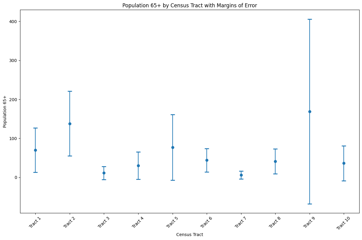
Visualization with Confidence Intervals

# Create error bar plot showing uncertainty
fig, ax = plt.subplots(figsize=(12, 8))

sample_data = ramsey_65plus.head(10)
x = range(len(sample_data))

ax.errorbar(
    x,
    sample_data["B01001_020E"],
    yerr=sample_data["moe_sum"],
    fmt="o",
    capsize=5,
    capthick=2,
)
ax.set_xlabel('Census Tract')
ax.set_ylabel('Population 65+')
ax.set_title('Population 65+ by Census Tract with Margins of Error')
plt.xticks(x, [f'Tract {i+1}' for i in x], rotation=45)
plt.tight_layout()
plt.show()