Simple Migration Flows with pytidycensus

This notebook demonstrates how to use the get_flows() function in pytidycensus to retrieve migration flow data from the Census Migration Flows API.

The Migration Flows API provides data on population movement between geographic areas based on American Community Survey (ACS) 5-year estimates.

import pytidycensus as tc
import pandas as pd
import matplotlib.pyplot as plt
import numpy as np
import pytidycensus as tc
import geopandas as gpd
import matplotlib.pyplot as plt
from shapely.geometry import LineString

# Set your Census API key
# tc.set_census_api_key("your_key_here")

Basic County-to-County Migration Flows

Let’s start with basic county-to-county migration flows for Texas:

# Get county-to-county migration flows for Texas
tx_flows = tc.get_flows(
    geography="county",
    state="TX",
    year=2018,
    output="wide"
)

print(f"Shape: {tx_flows.shape}")
print(f"Columns: {list(tx_flows.columns)}")
tx_flows.head()

Shape: (36641, 10)
Columns: ['GEOID1', 'GEOID2', 'FULL1_NAME', 'FULL2_NAME', 'MOVEDIN', 'MOVEDIN_M', 'MOVEDOUT', 'MOVEDOUT_M', 'MOVEDNET', 'MOVEDNET_M']

	GEOID1	GEOID2	FULL1_NAME	FULL2_NAME	MOVEDIN	MOVEDIN_M	MOVEDOUT	MOVEDOUT_M	MOVEDNET	MOVEDNET_M
0	48001	None	Anderson County, Texas	Africa	38	52.0	NaN	NaN	NaN	NaN
1	48001	None	Anderson County, Texas	Asia	4	6.0	NaN	NaN	NaN	NaN
2	48001	None	Anderson County, Texas	Central America	2	3.0	NaN	NaN	NaN	NaN
3	48001	01089	Anderson County, Texas	Madison County, Alabama	13	20.0	0.0	28.0	13.0	20.0
4	48001	02016	Anderson County, Texas	Aleutians West Census Area, Alaska	0	31.0	7.0	9.0	-7.0	9.0

Understanding the Data Structure

The flow data includes several key variables:

• MOVEDIN: Number of people who moved into the destination

• MOVEDOUT: Number of people who moved out of the origin

• MOVEDNET: Net migration (MOVEDIN - MOVEDOUT)

• FULL1_NAME: Origin location name

• FULL2_NAME: Destination location name

• Variables ending in _M: Margin of error

if geometry=True:

• centroid1: Origin centroid

• centroid2: Destination centroid

# Look at the largest migration flows
largest_flows = tx_flows.nlargest(10, 'MOVEDIN')
print("Top 10 largest migration flows:")
largest_flows[['FULL1_NAME', 'FULL2_NAME', 'MOVEDIN', 'MOVEDIN_M']].head()

Top 10 largest migration flows:

	FULL1_NAME	FULL2_NAME	MOVEDIN	MOVEDIN_M
12973	Fort Bend County, Texas	Harris County, Texas	20139	1842.0
30609	Tarrant County, Texas	Dallas County, Texas	19149	1603.0
10162	Denton County, Texas	Dallas County, Texas	18807	2114.0
15530	Harris County, Texas	Asia	18170	1557.0
6588	Collin County, Texas	Dallas County, Texas	17264	1567.0

Tidy Format for Analysis

The tidy format is better for analysis and visualization:

# Get the same data in tidy format
tx_flows_tidy = tc.get_flows(
    geography="county",
    state="TX", 
    year=2018,
    output="tidy"
)

print(f"Tidy format shape: {tx_flows_tidy.shape}")
tx_flows_tidy.head()

Tidy format shape: (109923, 7)

	GEOID1	GEOID2	FULL1_NAME	FULL2_NAME	variable	estimate	moe
0	48001	None	Anderson County, Texas	Africa	MOVEDIN	38.0	52.0
1	48001	None	Anderson County, Texas	Africa	MOVEDOUT	NaN	NaN
2	48001	None	Anderson County, Texas	Africa	MOVEDNET	NaN	NaN
3	48001	None	Anderson County, Texas	Asia	MOVEDIN	4.0	6.0
4	48001	None	Anderson County, Texas	Asia	MOVEDOUT	NaN	NaN

# Analyze migration patterns
migration_summary = tx_flows_tidy.groupby('variable')['estimate'].agg(['sum', 'mean', 'std'])
print("Migration flow summary:")
migration_summary

Migration flow summary:

	sum	mean	std
variable
MOVEDIN	1920233.0	52.406676	384.593025
MOVEDNET	130846.0	3.637744	147.398580
MOVEDOUT	1575040.0	43.788818	347.139862

Migration Flows with Demographic Breakdowns

Note: Breakdown characteristics are only available for years 2006-2015.

# Get flows with age and sex breakdowns (2015 data)
ri_flows_breakdown = tc.get_flows(
    geography="county",
    breakdown=["AGE", "SEX"],
    breakdown_labels=True,
    state="RI",
    year=2015,  # Breakdown only available before 2016
    output="tidy"
)

print(f"With breakdowns shape: {ri_flows_breakdown.shape}")
print(f"Breakdown columns: {[col for col in ri_flows_breakdown.columns if 'label' in col]}")
ri_flows_breakdown.head()

With breakdowns shape: (63072, 11)
Breakdown columns: ['AGE_label', 'SEX_label']

	GEOID1	GEOID2	FULL1_NAME	FULL2_NAME	AGE	SEX	AGE_label	SEX_label	variable	estimate	moe
0	44001	None	Bristol County, Rhode Island	Asia	00	00	All ages	All sexes	MOVEDIN	58.0	49.0
1	44001	None	Bristol County, Rhode Island	Asia	00	00	All ages	All sexes	MOVEDOUT	NaN	NaN
2	44001	None	Bristol County, Rhode Island	Asia	00	00	All ages	All sexes	MOVEDNET	NaN	NaN
3	44001	None	Bristol County, Rhode Island	Europe	00	00	All ages	All sexes	MOVEDIN	197.0	170.0
4	44001	None	Bristol County, Rhode Island	Europe	00	00	All ages	All sexes	MOVEDOUT	NaN	NaN

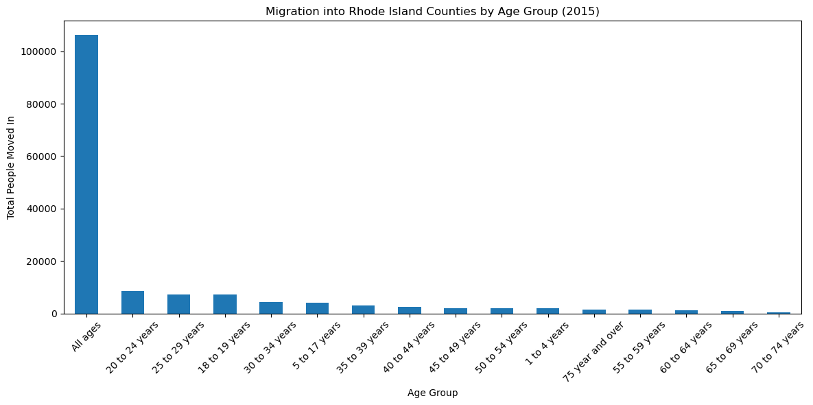
# Analyze migration by age group
if 'AGE_label' in ri_flows_breakdown.columns:
    age_migration = ri_flows_breakdown[ri_flows_breakdown['variable'] == 'MOVEDIN'].groupby('AGE_label')['estimate'].sum().sort_values(ascending=False)

    plt.figure(figsize=(12, 6))
    age_migration.plot(kind='bar')
    plt.title('Migration into Rhode Island Counties by Age Group (2015)')
    plt.xlabel('Age Group')
    plt.ylabel('Total People Moved In')
    plt.xticks(rotation=45)
    plt.tight_layout()
    plt.show()

Metropolitan Statistical Area Flows

Migration flows are also available at the MSA level (2013+):

# Get MSA-level migration flows
msa_flows = tc.get_flows(
    geography="metropolitan statistical area",
    year=2018,
    output="wide"
)

print(f"MSA flows shape: {msa_flows.shape}")
msa_flows.head()

MSA flows shape: (70428, 10)

	GEOID1	GEOID2	FULL1_NAME	FULL2_NAME	MOVEDIN	MOVEDIN_M	MOVEDOUT	MOVEDOUT_M	MOVEDNET	MOVEDNET_M
0	10180	None	Abilene, TX Metro Area	Outside Metro Area within U.S. or Puerto Rico	3883	508.0	2785.0	410.0	1098.0	684.0
1	10180	None	Abilene, TX Metro Area	Africa	134	152.0	NaN	NaN	NaN	NaN
2	10180	None	Abilene, TX Metro Area	Asia	504	207.0	NaN	NaN	NaN	NaN
3	10180	None	Abilene, TX Metro Area	Central America	56	42.0	NaN	NaN	NaN	NaN
4	10180	None	Abilene, TX Metro Area	Europe	264	176.0	NaN	NaN	NaN	NaN

# Find the largest MSA flows
largest_msa_flows = msa_flows.nlargest(10, 'MOVEDIN')
print("Largest MSA-to-MSA migration flows:")
for _, row in largest_msa_flows.iterrows():
    print(f"{row['FULL1_NAME']} > {row['FULL2_NAME']}: {row['MOVEDIN']:,} people")

Largest MSA-to-MSA migration flows:
Riverside-San Bernardino-Ontario, CA Metro Area > Los Angeles-Long Beach-Anaheim, CA Metro Area: 85,361 people
New York-Newark-Jersey City, NY-NJ-PA Metro Area > Asia: 65,239 people
Los Angeles-Long Beach-Anaheim, CA Metro Area > Asia: 57,528 people
Los Angeles-Long Beach-Anaheim, CA Metro Area > Riverside-San Bernardino-Ontario, CA Metro Area: 42,989 people
Dallas-Fort Worth-Arlington, TX Metro Area > Outside Metro Area within U.S. or Puerto Rico: 34,853 people
Philadelphia-Camden-Wilmington, PA-NJ-DE-MD Metro Area > New York-Newark-Jersey City, NY-NJ-PA Metro Area: 31,621 people
Washington-Arlington-Alexandria, DC-VA-MD-WV Metro Area > Asia: 31,025 people
Miami-Fort Lauderdale-West Palm Beach, FL Metro Area > Caribbean: 30,633 people
New York-Newark-Jersey City, NY-NJ-PA Metro Area > Europe: 29,904 people
San Francisco-Oakland-Hayward, CA Metro Area > Asia: 29,747 people

Margin of Error and Confidence Levels

You can adjust the confidence level for margin of error calculations:

# Compare different confidence levels
flows_90 = tc.get_flows(geography="county", state="NY", year=2018, moe_level=90, output="wide")
flows_95 = tc.get_flows(geography="county", state="NY", year=2018, moe_level=95, output="wide")
flows_99 = tc.get_flows(geography="county", state="NY", year=2018, moe_level=99, output="wide")

print("Margin of error comparison for first flow:")
print(f"90% confidence: {flows_90['MOVEDIN_M'].iloc[0]:.1f}")
print(f"95% confidence: {flows_95['MOVEDIN_M'].iloc[0]:.1f}") 
print(f"99% confidence: {flows_99['MOVEDIN_M'].iloc[0]:.1f}")

Margin of error comparison for first flow:
90% confidence: 33.0
95% confidence: 39.3
99% confidence: 51.4

Geometry Integration for Mapping

We automatically include shapely Point for the origin centroid1 and destination centroid2.

To help you install the required modules to help with plotting and webmaps please install:

pip install pytidycensus[map]

Here we add geographic centroids for mapping migration flows for Rhode Island:

# Get flows with geometry
flows_geo = tc.get_flows(
    geography="county",
    state="RI",
    year=2018,
    geometry=True,
    output="wide"
)
flows_geo.tail()

/home/mmann1123/Documents/github/pytidycensus/pytidycensus/flows.py:654: UserWarning: Could not find centroids for 9 GEOIDs: ['09011', '09013', '09001', '02261', '09009'].... These flows will not have geometry data.
  warnings.warn(

	GEOID1	GEOID2	FULL1_NAME	FULL2_NAME	MOVEDIN	MOVEDIN_M	MOVEDOUT	MOVEDOUT_M	MOVEDNET	MOVEDNET_M	centroid1	centroid2
1128	44009	55007	Washington County, Rhode Island	Bayfield County, Wisconsin	0	30.0	6.0	5.0	-6.0	5.0	POINT (-71.62272 41.46965)	POINT (-91.20137011438374 46.52300774226001)
1129	44009	55025	Washington County, Rhode Island	Dane County, Wisconsin	0	30.0	9.0	13.0	-9.0	13.0	POINT (-71.62272 41.46965)	POINT (-89.41818343109118 43.0673096742963)
1130	44009	55079	Washington County, Rhode Island	Milwaukee County, Wisconsin	0	30.0	14.0	23.0	-14.0	23.0	POINT (-71.62272 41.46965)	POINT (-87.96684239379597 43.00702311746134)
1131	44009	55101	Washington County, Rhode Island	Racine County, Wisconsin	36	56.0	0.0	20.0	36.0	56.0	POINT (-71.62272 41.46965)	POINT (-88.0613195061766 42.747515942441765)
1132	44009	72137	Washington County, Rhode Island	Toa Baja Municipio, Puerto Rico	2	3.0	0.0	32.0	2.0	3.0	POINT (-71.62272 41.46965)	POINT (-66.21454600086274 18.431092395056837)

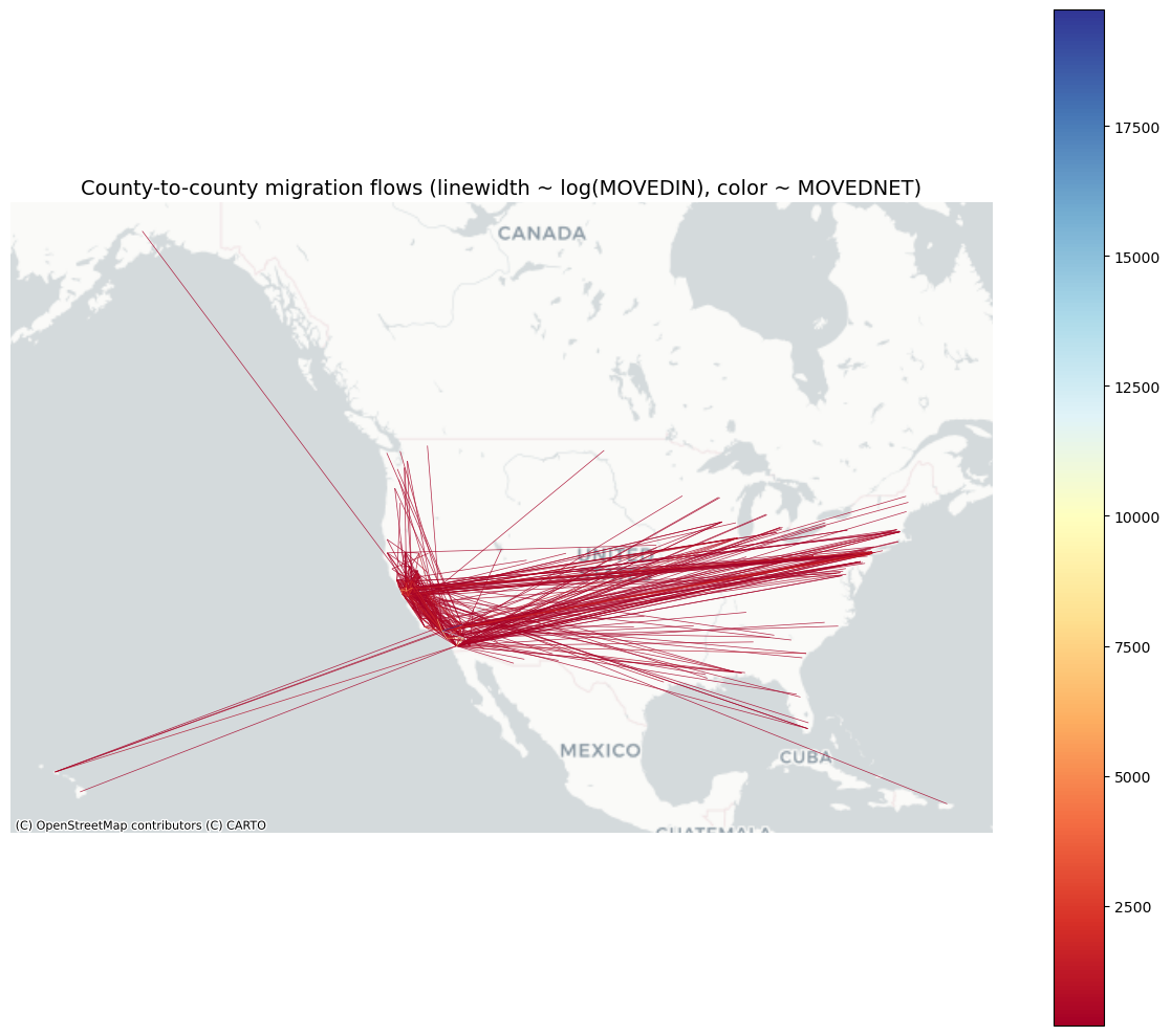
We can use those points to construct LineString to show flows on a map. Here we look a movements to and from California:

import pytidycensus as tc
import geopandas as gpd
import matplotlib.pyplot as plt
from shapely.geometry import LineString
import contextily as ctx 

# Get flows with geometry
flows_geo = tc.get_flows(
    geography="county",
    state="CA",
    year=2018,
    geometry=True,
    output="wide"
)

/home/mmann1123/Documents/github/pytidycensus/pytidycensus/flows.py:654: UserWarning: Could not find centroids for 115 GEOIDs: ['0900352140', '0901372090', '0901301080', '0901171670', '0900566420'].... These flows will not have geometry data.
  warnings.warn(

lines = flows_geo.copy()
lines = lines.dropna(subset=['centroid1', 'centroid2'])

lines['geometry'] = lines.apply(lambda r: LineString([r['centroid1'], r['centroid2']]) , axis=1)
lines = gpd.GeoDataFrame(lines, geometry='geometry', crs=flows_geo.crs)

# project to web mercator for basemap
lines_web = lines.to_crs(epsg=3857)

# dramatic width scaling: use log1p to increase contrast, then map to [min_w, max_w]
min_w, max_w = 0.5, 10.0
vals = np.log1p(lines_web['MOVEDIN'].astype(float).fillna(0))
max_val = vals.max() if vals.max() > 0 else 1.0
lines_web['lw'] = np.interp(vals, [0, max_val], [min_w, max_w])

# draw small flows first, large flows last (so large flows sit on top)
lines_web_sorted = lines_web.sort_values('MOVEDIN', ascending=True)

fig, ax = plt.subplots(figsize=(12, 10))
lines_web_sorted[lines_web_sorted['MOVEDNET'] > 200].plot(
    ax=ax,
    linewidth=lines_web_sorted['lw'],
    column='MOVEDNET',            # color by net migration
    cmap='RdYlBu',
    alpha=0.85,
    legend=True,
    zorder=1
)

# plot origin/destination centroids on top
orig_pts = gpd.GeoDataFrame(geometry=lines[['centroid1']].rename(columns={'centroid1':'geometry'})['geometry'], crs=lines.crs).set_geometry('geometry').to_crs(epsg=3857)
dest_pts = gpd.GeoDataFrame(geometry=lines[['centroid2']].rename(columns={'centroid2':'geometry'})['geometry'], crs=lines.crs).set_geometry('geometry').to_crs(epsg=3857)

# basemap with fallbacks
try:
    ctx.add_basemap(ax, source=ctx.providers.Stamen.TonerLite)
except Exception:
    try:
        ctx.add_basemap(ax, source=ctx.providers.CartoDB.Positron)
    except Exception:
        ctx.add_basemap(ax, source=ctx.providers.OpenStreetMap.Mapnik)

ax.set_axis_off()
plt.title('County-to-county migration flows (linewidth ~ log(MOVEDIN), color ~ MOVEDNET)', fontsize=14)
plt.tight_layout()
plt.show()

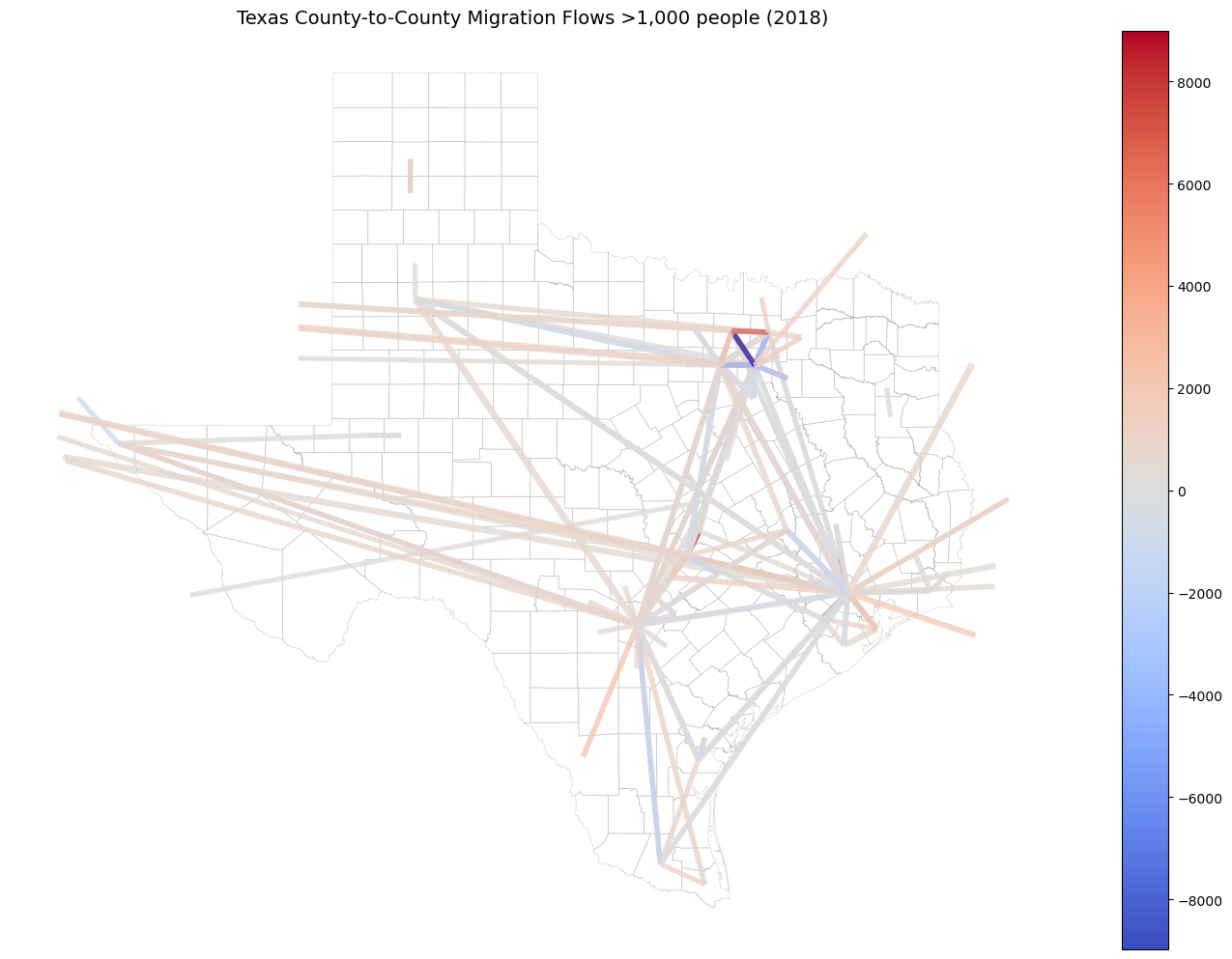
Simple Flow Map Without Basemap

For a cleaner look without external basemap dependencies:

import pytidycensus as tc
import geopandas as gpd
import matplotlib.pyplot as plt
from shapely.geometry import LineString
import numpy as np

# Get flows
flows_geo = tc.get_flows(
    geography="county",
    state="TX",
    year=2018,
    geometry=True,
    output="wide"
)

# Get Texas county boundaries for context
tx_counties = tc.get_geography("county", state="TX", year=2018)

# Create flow lines
lines = flows_geo.copy()
lines = lines.dropna(subset=['centroid1', 'centroid2'])
lines['geometry'] = lines.apply(lambda r: LineString([r['centroid1'], r['centroid2']]), axis=1)
lines = gpd.GeoDataFrame(lines, geometry='geometry', crs=flows_geo.crs)

# Filter significant flows
significant_flows = lines[lines['MOVEDIN'] > 1000].copy()

# Calculate line widths
min_w, max_w = 0.5, 5.0
vals = np.log1p(significant_flows['MOVEDIN'].astype(float))
max_val = vals.max() if vals.max() > 0 else 1.0
significant_flows['lw'] = np.interp(vals, [0, max_val], [min_w, max_w])

# Plot
fig, ax = plt.subplots(figsize=(14, 10))

# County boundaries as background
tx_counties.boundary.plot(ax=ax, linewidth=0.5, color='gray', alpha=0.3, zorder=1)
buf= tx_counties.geometry.buffer(0.5)

# Flow lines
significant_flows.clip(mask=buf).plot(
    ax=ax,
    linewidth=significant_flows['lw'],
    column='MOVEDNET',
    cmap='coolwarm',
    alpha=0.8,
    legend=True,
    zorder=2
)

ax.set_axis_off()
plt.title('Texas County-to-County Migration Flows >1,000 people (2018)', fontsize=14)
plt.tight_layout()
plt.show()

/home/mmann1123/Documents/github/pytidycensus/pytidycensus/flows.py:654: UserWarning: Could not find centroids for 97 GEOIDs: ['0900579510', '0900156060', '0901385950', '0900949950', '0900174190'].... These flows will not have geometry data.
  warnings.warn(
/tmp/ipykernel_54434/2996565908.py:39: UserWarning: Geometry is in a geographic CRS. Results from 'buffer' are likely incorrect. Use 'GeoSeries.to_crs()' to re-project geometries to a projected CRS before this operation.

  buf= tx_counties.geometry.buffer(0.5)

# ...existing code...
import folium
import branca.colormap as cm

# ensure numeric stroke width exists
significant_flows['lw'] = significant_flows['lw'].astype(float).fillna(1.0)

# folium expects GeoJSON in WGS84 (EPSG:4326)
gdf = significant_flows.drop(columns=['centroid1', 'centroid2'], errors='ignore').copy()
gjson = gdf.to_crs(epsg=4326).to_json()

# colormap for MOVEDNET
vmin = significant_flows['MOVEDNET'].min()
vmax = significant_flows['MOVEDNET'].max()
colormap = cm.LinearColormap(['#2166ac', '#ffffff', '#b2182b'], vmin=vmin, vmax=vmax)

def style_function(feature):
    props = feature.get('properties', {})
    lw = float(props.get('lw', 1.0))
    mv = props.get('MOVEDNET', 0)
    return {
        'weight': max(0.5, lw),                # ensure a minimum width
        'color': colormap(float(mv)) if mv is not None else '#888888',
        'opacity': 0.85
    }

# center map on data centroid (fallback coordinates provided)
centroid = significant_flows.geometry.unary_union.centroid
center = [centroid.y, centroid.x] if centroid is not None else [37.8, -96.9]

m = folium.Map(location=center, tiles='CartoDB positron', zoom_start=6)
folium.GeoJson(
    gjson,
    style_function=style_function,
    tooltip=folium.GeoJsonTooltip(fields=['FULL1_NAME', 'FULL2_NAME', 'MOVEDIN', 'MOVEDNET'])
).add_to(m)
colormap.caption = 'MOVEDNET'
colormap.add_to(m)

m
# ...existing code...

/tmp/ipykernel_54434/1650107880.py:28: DeprecationWarning: The 'unary_union' attribute is deprecated, use the 'union_all()' method instead.
  centroid = significant_flows.geometry.unary_union.centroid

Make this Notebook Trusted to load map: File -> Trust Notebook

Error Handling and Best Practices

Here are some common errors and how to handle them:

# Error: Invalid geography
try:
    tc.get_flows(geography="invalid", year=2018)
except ValueError as e:
    print(f"Geography error: {e}")

# Error: Year too early
try:
    tc.get_flows(geography="county", year=2009)
except ValueError as e:
    print(f"Year error: {e}")

# Error: Breakdown variables after 2015
try:
    tc.get_flows(geography="county", breakdown=["AGE"], year=2016)
except ValueError as e:
    print(f"Breakdown error: {e}")

# Error: MSA data before 2013
try:
    tc.get_flows(geography="metropolitan statistical area", year=2012)
except ValueError as e:
    print(f"MSA year error: {e}")

Geography error: Geography must be one of: county, county subdivision, metropolitan statistical area
Year error: Migration flows are available beginning in 2010
Breakdown error: Breakdown characteristics are only available for surveys before 2016
MSA year error: MSA-level data is only available beginning with 2013 (2009-2013 5-year ACS)

Summary

The get_flows() function provides comprehensive access to Census migration flow data with features including:

• Multiple geographic levels: county, county subdivision, MSA

• Flexible output formats: wide (API format) or tidy (analysis-ready)

• Demographic breakdowns: age, sex, race, income, etc. (2006-2015 only)

• Confidence levels: 90%, 95%, or 99% for margin of error

• Geometry integration: centroids for mapping flows

• Robust validation: comprehensive error checking and helpful messages

For more information, see the pytidycensus documentation.