Advanced Time Series Analysis: Handling Boundary Changes

This tutorial teaches advanced techniques for analyzing Census data over time when geographic boundaries change. You’ll learn to use area interpolation to handle census tract changes between 2019 and 2023 using ACS 5-year data.

What You’ll Learn

1. Area Interpolation: How to handle changing tract boundaries

2. Extensive vs Intensive Variables: Population counts vs poverty rates

3. Real-world Analysis: DC population and poverty trends (2019-2023)

4. Data Validation: Ensuring interpolation accuracy

5. Advanced Visualization: Mapping demographic change

Why Area Interpolation?

Census tract boundaries change periodically to:

• Maintain roughly equal population sizes (2,500-8,000 people)

• Reflect new development patterns

• Account for population shifts

Without interpolation: We can only compare tracts that didn’t change (loses data) With interpolation: We can analyze all areas by redistributing data from old to new boundaries

Setup: Install and Import Libraries

This tutorial requires additional spatial libraries beyond basic pytidycensus.

# Check if advanced spatial libraries are available
missing_packages = []

try:
    import geopandas as gpd
    print("geopandas available")
except ImportError:
    missing_packages.append('geopandas')
    print("geopandas missing")

try:
    from tobler.area_weighted import area_interpolate
    print("tobler available")
except ImportError:
    missing_packages.append('tobler')
    print("tobler missing")

if missing_packages:
    print(f"\nPlease install: pip install {' '.join(missing_packages)}")
    print("\nThese libraries are required for area interpolation.")
else:
    print("\nAll required libraries are available!")

geopandas available
tobler available

All required libraries are available!

# Import all required libraries
import pytidycensus as tc
import pandas as pd
import numpy as np
import matplotlib.pyplot as plt
import warnings
warnings.filterwarnings('ignore')

# Spatial libraries (if available)
try:
    import geopandas as gpd
    from tobler.area_weighted import area_interpolate
    SPATIAL_LIBS_AVAILABLE = True
except ImportError:
    SPATIAL_LIBS_AVAILABLE = False
    print("Spatial libraries not available - some features will be limited")

# Set up plotting style
plt.style.use('default')
plt.rcParams['figure.figsize'] = (15, 10)
plt.rcParams['font.size'] = 11

print("Libraries imported successfully!")
print(f"Using pytidycensus version: {tc.__version__}")
if SPATIAL_LIBS_AVAILABLE:
    print(f"Using geopandas version: {gpd.__version__}")

Libraries imported successfully!
Using pytidycensus version: 1.0.4
Using geopandas version: 1.1.1

# Set your Census API key
# Get a free key at: https://api.census.gov/data/key_signup.html

# UNCOMMENT and add your key:
# tc.set_census_api_key("YOUR_API_KEY_HERE")

print("Remember to set your Census API key above!")
print("This tutorial requires actual data downloads.")

Remember to set your Census API key above!
This tutorial requires actual data downloads.

Part 1: Understanding Boundary Changes

Let’s start by examining how census tract boundaries changed in Washington DC between 2019 and 2023 using ACS 5-year data.

# Step 1: Get 2019 ACS 5-year data with geometry
# This represents the 2015-2019 American Community Survey

try:
    dc_2019 = tc.get_acs(
        geography="tract",
        variables={
            "total_pop": "B01003_001E",      # Total population
            "poverty_count": "B17001_002E",  # Population below poverty line
            "poverty_total": "B17001_001E"   # Total population for poverty calculation
        },
        state="DC",
        year=2019,
        survey="acs5",
        geometry=True,  # Download tract boundaries
        output="wide"
    )
    
    # Calculate poverty rate
    dc_2019['poverty_rate'] = (dc_2019['poverty_count'] / dc_2019['poverty_total'] * 100)
    
    print(f"2019 ACS Data: {len(dc_2019)} tracts")
    print(f"Total population: {dc_2019['total_pop'].sum():,}")
    print(f"Average poverty rate: {dc_2019['poverty_rate'].mean():.1f}%")
    print(f"Coordinate system: {dc_2019.crs}")
    
except Exception as e:
    print(f"Error fetching 2019 data: {e}")
    dc_2019 = None

Getting data from the 2015-2019 5-year ACS
2019 ACS Data: 179 tracts
Total population: 692,683
Average poverty rate: 17.0%
Coordinate system: EPSG:4269

# Step 2: Get 2023 ACS 5-year data with geometry
# This represents the 2019-2023 American Community Survey

try:
    dc_2023 = tc.get_acs(
        geography="tract",
        variables={
            "total_pop": "B01003_001E",      # Total population
            "poverty_count": "B17001_002E",  # Population below poverty line
            "poverty_total": "B17001_001E"   # Total population for poverty calculation
        },
        state="DC",
        year=2023,
        survey="acs5",
        geometry=True,
        output="wide"
    )
    
    # Calculate poverty rate
    dc_2023['poverty_rate'] = (dc_2023['poverty_count'] / dc_2023['poverty_total'] * 100)
    
    print(f"2023 ACS Data: {len(dc_2023)} tracts")
    print(f"Total population: {dc_2023['total_pop'].sum():,}")
    print(f"Average poverty rate: {dc_2023['poverty_rate'].mean():.1f}%")
    print(f"Coordinate system: {dc_2023.crs}")
    
    # Check for boundary changes
    if dc_2019 is not None:
        tract_change = len(dc_2023) - len(dc_2019)
        print(f"\nBoundary Changes:")
        print(f"Tract count change: {tract_change:+d}")
        
        # Check for common tracts
        common_tracts = set(dc_2019['GEOID']) & set(dc_2023['GEOID'])
        print(f"Unchanged tracts: {len(common_tracts)}")
        print(f"Changed/new tracts: {len(dc_2023) - len(common_tracts)}")
        
except Exception as e:
    print(f"Error fetching 2023 data: {e}")
    dc_2023 = None

Getting data from the 2019-2023 5-year ACS
2023 ACS Data: 206 tracts
Total population: 672,079
Average poverty rate: 15.6%
Coordinate system: EPSG:4269

Boundary Changes:
Tract count change: +27
Unchanged tracts: 154
Changed/new tracts: 52

NOTE: There were 52 new or changed tracts in DC between 2019 and 2023.

Visualizing Boundary Changes

Let’s create maps to visualize how tract boundaries changed between 2019 and 2023, and see the differences in both population and poverty patterns.

# Create boundary comparison maps
if dc_2019 is not None and dc_2023 is not None:
    fig, ((ax1, ax2), (ax3, ax4)) = plt.subplots(2, 2, figsize=(20, 16))
    
    # 2019 Population
    dc_2019.plot(
        column='total_pop',
        cmap='Blues',
        legend=True,
        ax=ax1,
        edgecolor='white',
        linewidth=0.5,
        legend_kwds={'label': 'Total Population', 'shrink': 0.8}
    )
    ax1.set_title('2019 ACS 5-year: Total Population\n(2015-2019 Data)', fontsize=14, fontweight='bold')
    ax1.axis('off')
    
    # 2023 Population
    dc_2023.plot(
        column='total_pop',
        cmap='Blues',
        legend=True,
        ax=ax2,
        edgecolor='white',
        linewidth=0.5,
        legend_kwds={'label': 'Total Population', 'shrink': 0.8}
    )
    ax2.set_title('2023 ACS 5-year: Total Population\n(2019-2023 Data)', fontsize=14, fontweight='bold')
    ax2.axis('off')
    
    # 2019 Poverty Rate
    dc_2019.plot(
        column='poverty_rate',
        cmap='Reds',
        legend=True,
        ax=ax3,
        edgecolor='white',
        linewidth=0.5,
        vmin=0,
        vmax=50,
        legend_kwds={'label': 'Poverty Rate (%)', 'shrink': 0.8}
    )
    ax3.set_title('2019 ACS 5-year: Poverty Rate\n(2015-2019 Data)', fontsize=14, fontweight='bold')
    ax3.axis('off')
    
    # 2023 Poverty Rate
    dc_2023.plot(
        column='poverty_rate',
        cmap='Reds',
        legend=True,
        ax=ax4,
        edgecolor='white',
        linewidth=0.5,
        vmin=0,
        vmax=50,
        legend_kwds={'label': 'Poverty Rate (%)', 'shrink': 0.8}
    )
    ax4.set_title('2023 ACS 5-year: Poverty Rate\n(2019-2023 Data)', fontsize=14, fontweight='bold')
    ax4.axis('off')
    
    plt.tight_layout()
    plt.suptitle('Census Tract Boundaries and Variables: 2019 vs 2023', 
                 fontsize=18, fontweight='bold', y=.96)
    plt.show()
    
else:
    print("Cannot create boundary comparison - missing data")
    print("This tutorial works best with working API key and data access")

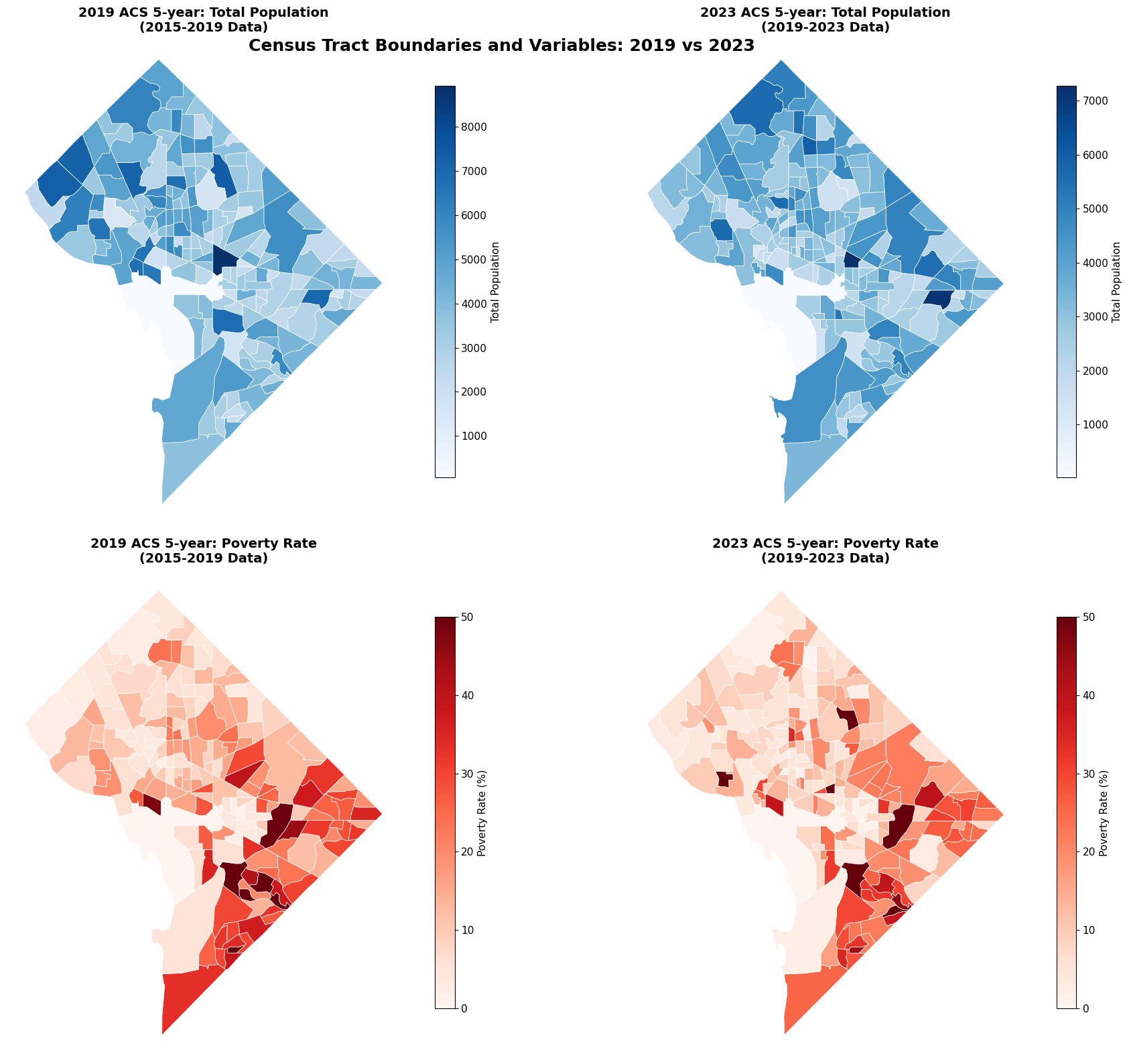
Key Insight: Why Interpolation is Needed

Notice how the number of tracts and their boundaries may have changed between 2019 and 2023. Some tracts were:

• Split: One tract became multiple tracts

• Merged: Multiple tracts became one tract

• Renumbered: Same area, different GEOID

• Boundary adjusted: Slight changes to tract edges

Without interpolation, we could only analyze the tracts that remained exactly the same!

Part 2: Coordinate Reference Systems for Area Calculations

Before performing area interpolation, we need to understand coordinate reference systems (CRS). This is crucial for accurate area calculations.

if dc_2019 is not None and dc_2023 is not None:
    print("COORDINATE REFERENCE SYSTEMS")
    print("=" * 50)
    print(f"Original CRS: {dc_2019.crs}")
    print("   • EPSG:4326 = Geographic coordinates (latitude/longitude)")
    print("   • Good for: Mapping, display")
    print("   • Bad for: Area calculations (distorted)")
    print()
    
    # Transform to projected coordinate system for area calculations
    print("Transforming to projected coordinate system...")
    dc_2019_proj = dc_2019.to_crs('EPSG:3857')  # Web Mercator
    dc_2023_proj = dc_2023.to_crs('EPSG:3857')
    
    print(f"Projected CRS: {dc_2019_proj.crs}")
    print("   • EPSG:3857 = Web Mercator (projected coordinates)")
    print("   • Good for: Area calculations, spatial analysis")
    print("   • Bad for: High-latitude areas (less accurate)")
    print()
    
    # Demonstrate the difference
    sample_tract_geo = dc_2019.iloc[0:1]
    sample_tract_proj = dc_2019_proj.iloc[0:1]
    
    area_geo = sample_tract_geo.area.iloc[0]  # In degrees^2 (meaningless)
    area_proj = sample_tract_proj.area.iloc[0]  # In meters^2 (meaningful)
    
    print(f"AREA CALCULATION EXAMPLE:")
    print(f"   Geographic (EPSG:4326): {area_geo:.8f} degrees²")
    print(f"   Projected (EPSG:3857): {area_proj:.0f} meters²")
    print(f"   Projected in acres: {area_proj * 0.000247:.1f} acres")
    print()
    print("Key Learning: Always use projected coordinates for spatial analysis!")
    
else:
    print("Need data to demonstrate coordinate systems")
    # Create dummy projected variables for later code
    dc_2019_proj = None
    dc_2023_proj = None

COORDINATE REFERENCE SYSTEMS
==================================================
Original CRS: EPSG:4269
   • EPSG:4326 = Geographic coordinates (latitude/longitude)
   • Good for: Mapping, display
   • Bad for: Area calculations (distorted)

Transforming to projected coordinate system...
Projected CRS: EPSG:3857
   • EPSG:3857 = Web Mercator (projected coordinates)
   • Good for: Area calculations, spatial analysis
   • Bad for: High-latitude areas (less accurate)

AREA CALCULATION EXAMPLE:
   Geographic (EPSG:4326): 0.00006818 degrees²
   Projected (EPSG:3857): 1086381 meters²
   Projected in acres: 268.3 acres

Key Learning: Always use projected coordinates for spatial analysis!

Part 3: Extensive vs Intensive Variables

Understanding variable types is crucial for proper interpolation:

• Extensive variables: Counts/totals that should be summed when areas are combined

• Intensive variables: Rates/ratios that should be averaged when areas are combined

The interpolation algorithm handles these differently!

Variable Classification for Our Analysis

Extensive Variables (Counts - use area-weighted SUM):

• Total population (total_pop)

• Number of people in poverty (poverty_count)

• Total population for poverty calculation (poverty_total)

Intensive Variables (Rates - use area-weighted AVERAGE):

• Poverty rate (poverty_rate) - percentage of people below poverty line

Example: Combining Two Census Tracts

Tract A: 1,000 people, 20% poverty rate (200 people in poverty) Tract B: 2,000 people, 10% poverty rate (200 people in poverty)

Correct way to combine:

• Total population: 1,000 + 2,000 = 3,000 (SUM)

• People in poverty: 200 + 200 = 400 (SUM)

• Poverty rate: 400 / 3,000 = 13.3% (WEIGHTED AVERAGE)

Wrong way:

• Poverty rate: (20% + 10%) / 2 = 15% (SIMPLE AVERAGE)

Area interpolation handles this automatically when you classify variables correctly!

Part 4: Performing Area Interpolation

Now let’s perform the actual area interpolation to redistribute 2019 data to 2023 tract boundaries.

# Perform area interpolation
if SPATIAL_LIBS_AVAILABLE and dc_2019_proj is not None and dc_2023_proj is not None:
    print("PERFORMING AREA INTERPOLATION")
    print("=" * 50)
    print("This process:")
    print("  1. Projects data to appropriate coordinate system")
    print("  2. Overlays 2019 tracts onto 2023 tracts")
    print("  3. Calculates intersection areas")
    print("  4. Redistributes data proportionally")
    print()
    
    # Define variable types for interpolation
    extensive_variables = ['total_pop', 'poverty_count', 'poverty_total']  # Counts (sum)
    intensive_variables = ['poverty_rate']                                 # Rates (weighted average)
    
    print(f"Variable Classification:")
    print(f"   Extensive (counts): {extensive_variables}")
    print(f"   Intensive (rates): {intensive_variables}")
    print()
    
    # Perform interpolation
    print("Running area_interpolate...")
    try:
        dc_2019_interpolated = area_interpolate(
            source_df=dc_2019_proj,              # 2019 data (source)
            target_df=dc_2023_proj,              # 2023 boundaries (target) 
            extensive_variables=extensive_variables,
            intensive_variables=intensive_variables
        )
        
        print("Interpolation complete!")
        print()
        
        # Validation
        print("VALIDATION RESULTS:")
        
        # Check population conservation for extensive variables
        orig_pop = dc_2019['total_pop'].sum()
        interp_pop = dc_2019_interpolated['total_pop'].sum()
        pop_difference = abs(orig_pop - interp_pop)
        
        orig_poverty_count = dc_2019['poverty_count'].sum()
        interp_poverty_count = dc_2019_interpolated['poverty_count'].sum()
        poverty_difference = abs(orig_poverty_count - interp_poverty_count)
        
        print(f"Population Conservation:")
        print(f"   Original 2019 population: {orig_pop:,}")
        print(f"   Interpolated population: {interp_pop:,.0f}")
        print(f"   Difference: {pop_difference:,.0f} ({pop_difference/orig_pop*100:.3f}%)")
        print()
        
        print(f"Poverty Count Conservation:")
        print(f"   Original poverty count: {orig_poverty_count:,}")
        print(f"   Interpolated poverty count: {interp_poverty_count:,.0f}")
        print(f"   Difference: {poverty_difference:,.0f} ({poverty_difference/orig_poverty_count*100:.3f}%)")
        print()
        
        # Check poverty rate consistency
        orig_avg_rate = dc_2019['poverty_rate'].mean()
        interp_avg_rate = dc_2019_interpolated['poverty_rate'].mean()
        rate_difference = abs(orig_avg_rate - interp_avg_rate)
        
        print(f"Poverty Rate Consistency:")
        print(f"   Original average rate: {orig_avg_rate:.2f}%")
        print(f"   Interpolated average rate: {interp_avg_rate:.2f}%")
        print(f"   Difference: {rate_difference:.3f} percentage points")
        print()
        
        print("Small differences are normal due to edge effects and rounding.")
        
    except Exception as e:
        print(f"Interpolation failed: {e}")
        dc_2019_interpolated = None
        
else:
    print("Area interpolation requires:")
    print("   • tobler library (pip install tobler)")
    print("   • geopandas library (pip install geopandas)")
    print("   • Working Census API key")
    print("   • Successful data downloads")
    dc_2019_interpolated = None

PERFORMING AREA INTERPOLATION
==================================================
This process:
  1. Projects data to appropriate coordinate system
  2. Overlays 2019 tracts onto 2023 tracts
  3. Calculates intersection areas
  4. Redistributes data proportionally

Variable Classification:
   Extensive (counts): ['total_pop', 'poverty_count', 'poverty_total']
   Intensive (rates): ['poverty_rate']

Running area_interpolate...
Interpolation complete!

VALIDATION RESULTS:
Population Conservation:
   Original 2019 population: 692,683
   Interpolated population: 692,683
   Difference: 0 (0.000%)

Poverty Count Conservation:
   Original poverty count: 107,140
   Interpolated poverty count: 107,140
   Difference: 0 (0.000%)

Poverty Rate Consistency:
   Original average rate: 17.01%
   Interpolated average rate: 16.27%
   Difference: 0.746 percentage points

Small differences are normal due to edge effects and rounding.

Understanding Interpolation Results

The interpolation process:

1. Overlays old tract boundaries on new tract boundaries

2. Calculates the area of each intersection

3. Redistributes data proportionally based on area overlap

4. Preserves total counts while properly weighting rates

Small differences in totals are normal due to:

• Edge effects at boundaries

• Rounding in calculations

• Slight changes in total area due to map projections

Part 5: Calculate Changes Using Interpolated Data

# Calculate changes using interpolated data
if dc_2019_interpolated is not None and dc_2023_proj is not None:
    print("CALCULATING CHANGES (2019-2023)")
    print("=" * 50)
    
    # Create change analysis dataset using 2023 boundaries
    dc_change = dc_2023_proj.copy()
    
    # Add interpolated 2019 data
    dc_change['total_pop_2019'] = dc_2019_interpolated['total_pop']
    dc_change['poverty_rate_2019'] = dc_2019_interpolated['poverty_rate']
    dc_change['poverty_count_2019'] = dc_2019_interpolated['poverty_count']
    
    # Add 2023 data (already in the dataset)
    dc_change['total_pop_2023'] = dc_2023_proj['total_pop']
    dc_change['poverty_rate_2023'] = dc_2023_proj['poverty_rate']
    dc_change['poverty_count_2023'] = dc_2023_proj['poverty_count']
    
    # Calculate changes
    dc_change['pop_change'] = dc_change['total_pop_2023'] - dc_change['total_pop_2019']
    dc_change['pop_change_pct'] = (dc_change['pop_change'] / dc_change['total_pop_2019']) * 100
    dc_change['poverty_rate_change'] = dc_change['poverty_rate_2023'] - dc_change['poverty_rate_2019']
    dc_change['poverty_count_change'] = dc_change['poverty_count_2023'] - dc_change['poverty_count_2019']
    
    # Summary statistics
    total_pop_change = dc_change['pop_change'].sum()
    avg_poverty_rate_change = dc_change['poverty_rate_change'].mean()
    total_poverty_count_change = dc_change['poverty_count_change'].sum()
    
    tracts_pop_growing = (dc_change['pop_change'] > 50).sum()  # >50 person increase
    tracts_pop_declining = (dc_change['pop_change'] < -50).sum()  # >50 person decrease
    tracts_poverty_improving = (dc_change['poverty_rate_change'] < -1).sum()  # >1pp decrease
    tracts_poverty_worsening = (dc_change['poverty_rate_change'] > 1).sum()   # >1pp increase
    
    print(f"POPULATION CHANGE ANALYSIS:")
    print(f"   Total population change: {total_pop_change:+,.0f} people")
    print(f"   Tracts with population growth (>50): {tracts_pop_growing}")
    print(f"   Tracts with population decline (>50): {tracts_pop_declining}")
    print()
    print(f"POVERTY CHANGE ANALYSIS:")
    print(f"   Average poverty rate change: {avg_poverty_rate_change:+.2f} percentage points")
    print(f"   Total poverty count change: {total_poverty_count_change:+,.0f} people")
    print(f"   Tracts improving (>1pp decrease): {tracts_poverty_improving}")
    print(f"   Tracts worsening (>1pp increase): {tracts_poverty_worsening}")
    
else:
    print("Cannot calculate changes - missing interpolation results")
    dc_change = None

CALCULATING CHANGES (2019-2023)
==================================================
POPULATION CHANGE ANALYSIS:
   Total population change: -20,604 people
   Tracts with population growth (>50): 67
   Tracts with population decline (>50): 128

POVERTY CHANGE ANALYSIS:
   Average poverty rate change: -0.70 percentage points
   Total poverty count change: -13,000 people
   Tracts improving (>1pp decrease): 107
   Tracts worsening (>1pp increase): 71

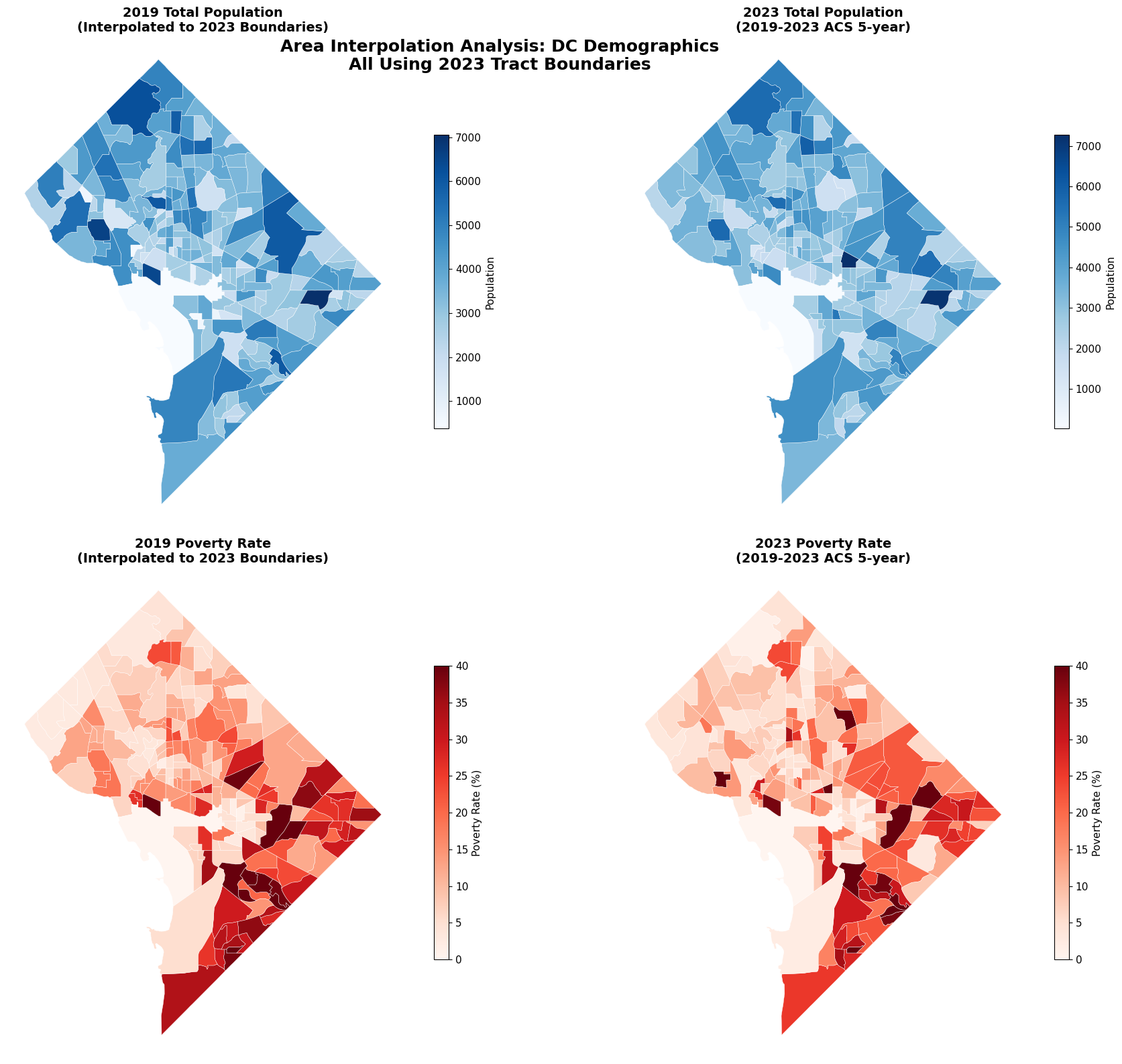
Part 6: Advanced Visualization of Changes

Let’s create comprehensive visualizations that show both the original data and the changes over time, all using the consistent 2023 tract boundaries.

# Create comprehensive change visualization
if dc_change is not None:
    # Convert back to geographic coordinates for mapping
    dc_change_geo = dc_change.to_crs('EPSG:4326')
    
    fig, ((ax1, ax2), (ax3, ax4)) = plt.subplots(2, 2, figsize=(20, 16))
    
    # Map 1: 2019 Population (Interpolated to 2023 boundaries)
    dc_change_geo.plot(
        column='total_pop_2019',
        cmap='Blues',
        legend=True,
        ax=ax1,
        edgecolor='white',
        linewidth=0.3,
        legend_kwds={'label': 'Population', 'shrink': 0.6}
    )
    ax1.set_title('2019 Total Population\n(Interpolated to 2023 Boundaries)', 
                  fontsize=14, fontweight='bold')
    ax1.axis('off')
    
    # Map 2: 2023 Population
    dc_change_geo.plot(
        column='total_pop_2023',
        cmap='Blues',
        legend=True,
        ax=ax2,
        edgecolor='white',
        linewidth=0.3,
        legend_kwds={'label': 'Population', 'shrink': 0.6}
    )
    ax2.set_title('2023 Total Population\n(2019-2023 ACS 5-year)', 
                  fontsize=14, fontweight='bold')
    ax2.axis('off')
    
    # Map 3: 2019 Poverty Rate (Interpolated)
    dc_change_geo.plot(
        column='poverty_rate_2019',
        cmap='Reds',
        legend=True,
        ax=ax3,
        edgecolor='white',
        linewidth=0.3,
        vmin=0,
        vmax=40,
        legend_kwds={'label': 'Poverty Rate (%)', 'shrink': 0.6}
    )
    ax3.set_title('2019 Poverty Rate\n(Interpolated to 2023 Boundaries)', 
                  fontsize=14, fontweight='bold')
    ax3.axis('off')
    
    # Map 4: 2023 Poverty Rate
    dc_change_geo.plot(
        column='poverty_rate_2023',
        cmap='Reds',
        legend=True,
        ax=ax4,
        edgecolor='white',
        linewidth=0.3,
        vmin=0,
        vmax=40,
        legend_kwds={'label': 'Poverty Rate (%)', 'shrink': 0.6}
    )
    ax4.set_title('2023 Poverty Rate\n(2019-2023 ACS 5-year)', 
                  fontsize=14, fontweight='bold')
    ax4.axis('off')
    
    plt.tight_layout()
    plt.suptitle('Area Interpolation Analysis: DC Demographics\nAll Using 2023 Tract Boundaries', 
                 fontsize=18, fontweight='bold', y=0.96)
    plt.show()
    
else:
    print("Cannot create advanced visualization - missing change data")

# Create change-focused visualization
if dc_change is not None:
    fig, ((ax1, ax2), (ax3, ax4)) = plt.subplots(2, 2, figsize=(20, 16))
    
    # Map 1: Population Change (Absolute)
    dc_change_geo.plot(
        column='pop_change',
        cmap='RdBu_r',
        legend=True,
        ax=ax1,
        edgecolor='white',
        linewidth=0.3,
        legend_kwds={'label': 'Population Change', 'shrink': 0.6}
    )
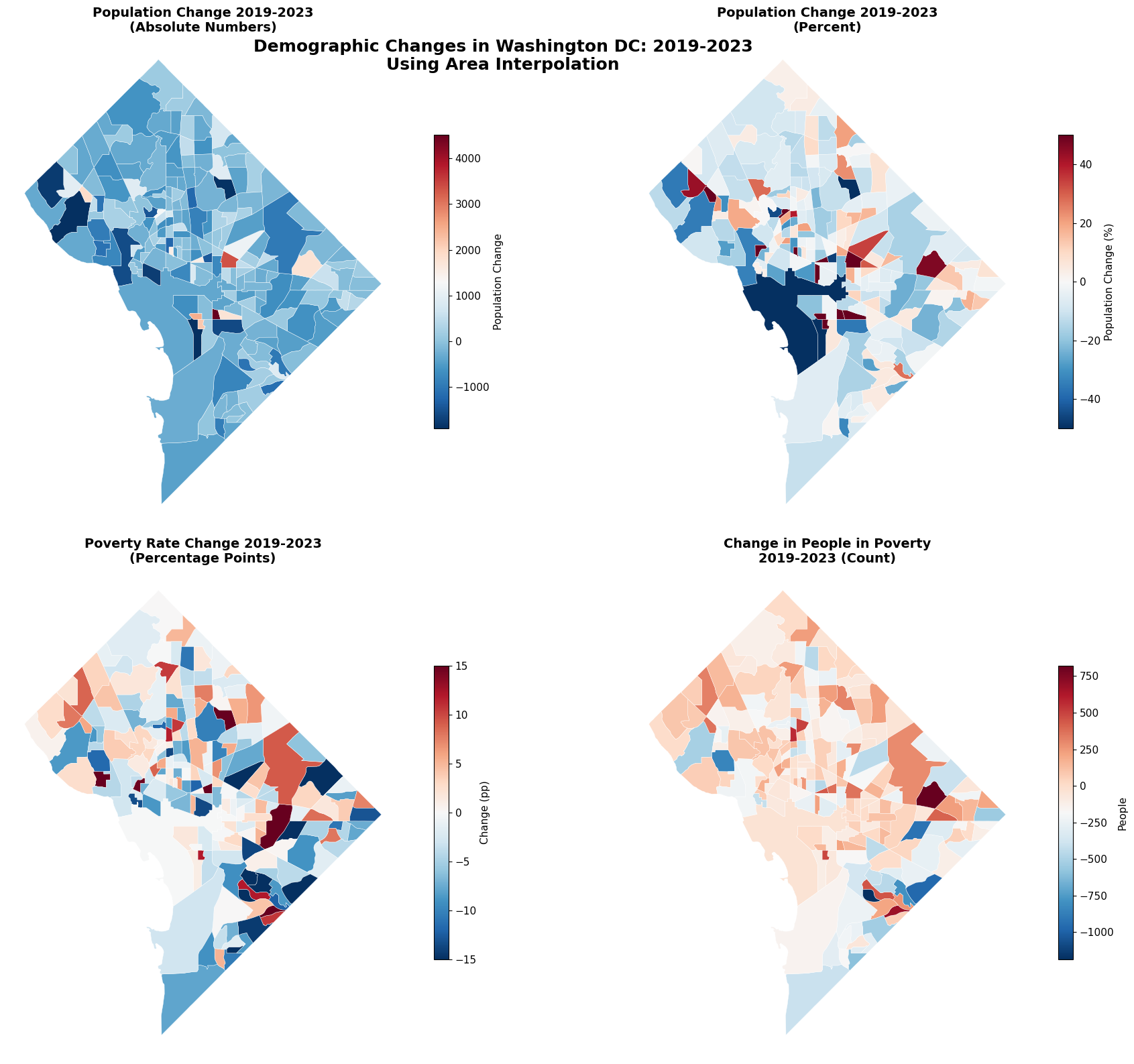
    ax1.set_title('Population Change 2019-2023\n(Absolute Numbers)', 
                  fontsize=14, fontweight='bold')
    ax1.axis('off')
    
    # Map 2: Population Change (Percent)
    # Handle infinite values
    pop_change_pct_clean = dc_change_geo['pop_change_pct'].replace([np.inf, -np.inf], np.nan)
    dc_change_geo_temp = dc_change_geo.copy()
    dc_change_geo_temp['pop_change_pct_clean'] = pop_change_pct_clean
    
    dc_change_geo_temp.plot(
        column='pop_change_pct_clean',
        cmap='RdBu_r',
        legend=True,
        ax=ax2,
        edgecolor='white',
        linewidth=0.3,
        vmin=-50,
        vmax=50,
        legend_kwds={'label': 'Population Change (%)', 'shrink': 0.6}
    )
    ax2.set_title('Population Change 2019-2023\n(Percent)', 
                  fontsize=14, fontweight='bold')
    ax2.axis('off')
    
    # Map 3: Poverty Rate Change
    dc_change_geo.plot(
        column='poverty_rate_change',
        cmap='RdBu_r',
        legend=True,
        ax=ax3,
        edgecolor='white',
        linewidth=0.3,
        vmin=-15,
        vmax=15,
        legend_kwds={'label': 'Change (pp)', 'shrink': 0.6}
    )
    ax3.set_title('Poverty Rate Change 2019-2023\n(Percentage Points)', 
                  fontsize=14, fontweight='bold')
    ax3.axis('off')
    
    # Map 4: Poverty Count Change
    dc_change_geo.plot(
        column='poverty_count_change',
        cmap='RdBu_r',
        legend=True,
        ax=ax4,
        edgecolor='white',
        linewidth=0.3,
        legend_kwds={'label': 'People', 'shrink': 0.6}
    )
    ax4.set_title('Change in People in Poverty\n2019-2023 (Count)', 
                  fontsize=14, fontweight='bold')
    ax4.axis('off')
    
    plt.tight_layout()
    plt.suptitle('Demographic Changes in Washington DC: 2019-2023\nUsing Area Interpolation', 
                 fontsize=18, fontweight='bold', y=0.96)
    plt.show()
    
    print("INTERPRETING THE MAPS:")
    print("   • Red areas: Higher values or increases")
    print("   • Blue areas: Lower values or decreases")
    print("   • White areas: No data or minimal change")
    print("   • All maps use the same 2023 tract boundaries for direct comparison")
    
else:
    print("Cannot create change visualization - missing data")

INTERPRETING THE MAPS:
   • Red areas: Higher values or increases
   • Blue areas: Lower values or decreases
   • White areas: No data or minimal change
   • All maps use the same 2023 tract boundaries for direct comparison

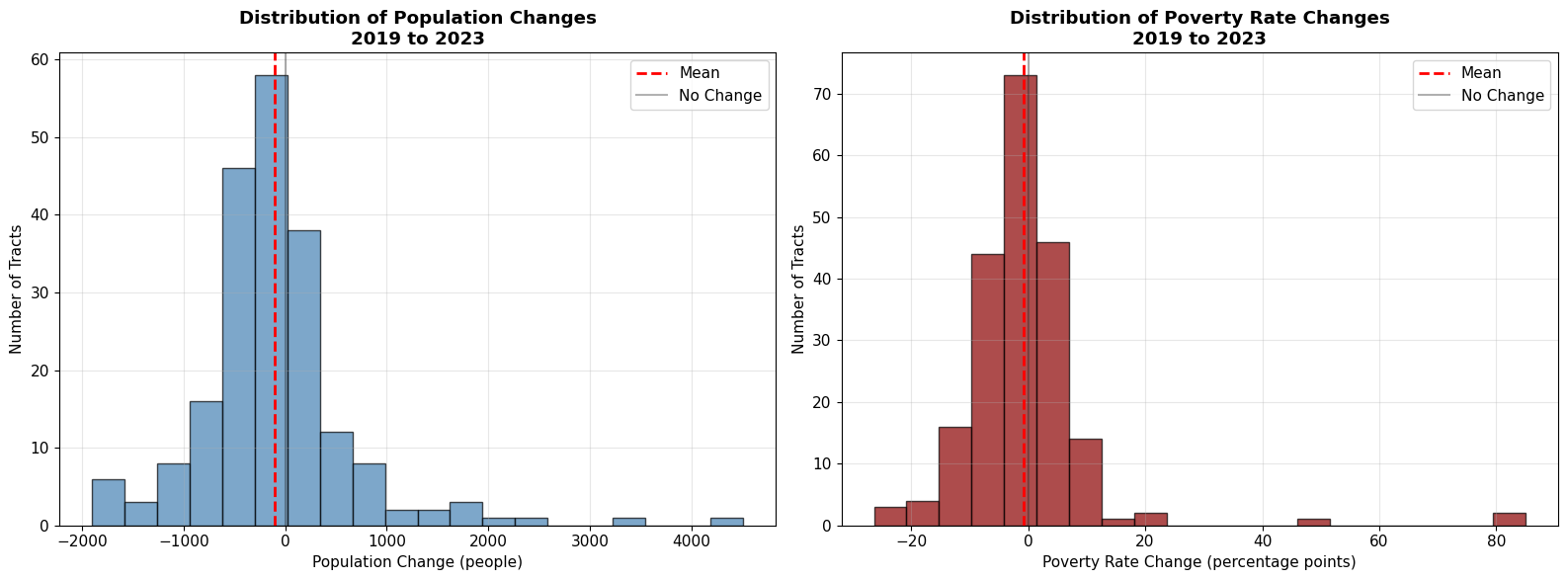
Part 7: Statistical Analysis and Validation

Let’s dig deeper into the patterns we observed and validate our interpolation results.

# Statistical analysis of changes
if dc_change is not None:
    print("DETAILED STATISTICAL ANALYSIS")
    print("=" * 60)
    
    # Population change distribution
    print(f"POPULATION CHANGES:")
    print(f"   Mean change: {dc_change['pop_change'].mean():+.0f} people")
    print(f"   Median change: {dc_change['pop_change'].median():+.0f} people")
    print(f"   Std deviation: {dc_change['pop_change'].std():.0f}")
    print(f"   Range: {dc_change['pop_change'].min():+.0f} to {dc_change['pop_change'].max():+.0f}")
    print()
    
    # Poverty rate change distribution
    print(f"POVERTY RATE CHANGES (percentage points):")
    print(f"   Mean: {dc_change['poverty_rate_change'].mean():+.2f}")
    print(f"   Median: {dc_change['poverty_rate_change'].median():+.2f}")
    print(f"   Std deviation: {dc_change['poverty_rate_change'].std():.2f}")
    print(f"   Range: {dc_change['poverty_rate_change'].min():+.1f} to {dc_change['poverty_rate_change'].max():+.1f}")
    print()
    
    # Create histograms
    fig, (ax1, ax2) = plt.subplots(1, 2, figsize=(16, 6))
    
    # Population change histogram
    ax1.hist(dc_change['pop_change'], bins=20, alpha=0.7, color='steelblue', edgecolor='black')
    ax1.axvline(dc_change['pop_change'].mean(), color='red', linestyle='--', linewidth=2, label='Mean')
    ax1.axvline(0, color='black', linestyle='-', alpha=0.3, label='No Change')
    ax1.set_xlabel('Population Change (people)')
    ax1.set_ylabel('Number of Tracts')
    ax1.set_title('Distribution of Population Changes\n2019 to 2023', fontweight='bold')
    ax1.legend()
    ax1.grid(True, alpha=0.3)
    
    # Poverty rate change histogram
    ax2.hist(dc_change['poverty_rate_change'], bins=20, alpha=0.7, color='darkred', edgecolor='black')
    ax2.axvline(dc_change['poverty_rate_change'].mean(), color='red', linestyle='--', linewidth=2, label='Mean')
    ax2.axvline(0, color='black', linestyle='-', alpha=0.3, label='No Change')
    ax2.set_xlabel('Poverty Rate Change (percentage points)')
    ax2.set_ylabel('Number of Tracts')
    ax2.set_title('Distribution of Poverty Rate Changes\n2019 to 2023', fontweight='bold')
    ax2.legend()
    ax2.grid(True, alpha=0.3)
    
    plt.tight_layout()
    plt.show()
    
else:
    print("Cannot perform statistical analysis - missing data")

DETAILED STATISTICAL ANALYSIS
============================================================
POPULATION CHANGES:
   Mean change: -100 people
   Median change: -148 people
   Std deviation: 775
   Range: -1907 to +4512

POVERTY RATE CHANGES (percentage points):
   Mean: -0.70
   Median: -1.23
   Std deviation: 11.49
   Range: -26.4 to +85.0

Part 8: Best Practices and Limitations

When to Use Area Interpolation

Appropriate uses:

• Comparing small geographies across census years

• Geographic boundaries have changed

• You need comprehensive spatial coverage

• Data is reasonably evenly distributed within areas

When not to use:

• Analyzing point locations (schools, businesses)

• Data is highly concentrated in specific areas

• Geography hasn’t changed (use simple comparison)

• Very small sample sizes (ACS margins of error too large)

Methodology Best Practices

1. Always use projected coordinate systems (e.g., EPSG:3857)

2. Classify variables correctly (extensive vs intensive)

3. Validate interpolation results thoroughly

4. Document your assumptions and limitations

5. Consider alternative approaches (relationship files)

Important Limitations

• Assumes uniform distribution within source areas

• Edge effects can create small errors

• Not appropriate for highly clustered phenomena

• Results are estimates, not exact values

• Works best with areally extensive data

Summary: What You’ve Accomplished

Technical Skills Mastered

1. Area Interpolation: Redistributing data across changing boundaries using tobler.area_interpolate()

2. Variable Classification: Properly handling extensive (counts) vs intensive (rates) variables

3. Coordinate Systems: Using projected CRS (EPSG:3857) for accurate area calculations

4. Data Validation: Checking interpolation accuracy through conservation tests

5. Advanced Visualization: Creating comprehensive maps showing both original data and changes

Additional Resources

• Tobler Documentation - Complete guide to spatial interpolation

• Census Relationship Files - Official boundary change documentation

• PySAL Spatial Analysis - Advanced spatial analysis tools

• Dasymetric Mapping Literature - Advanced interpolation techniques

You now have the skills to conduct sophisticated temporal analysis of Census data while properly handling the complex issue of changing geographic boundaries. This methodology enables robust longitudinal research that maintains spatial consistency across time periods.